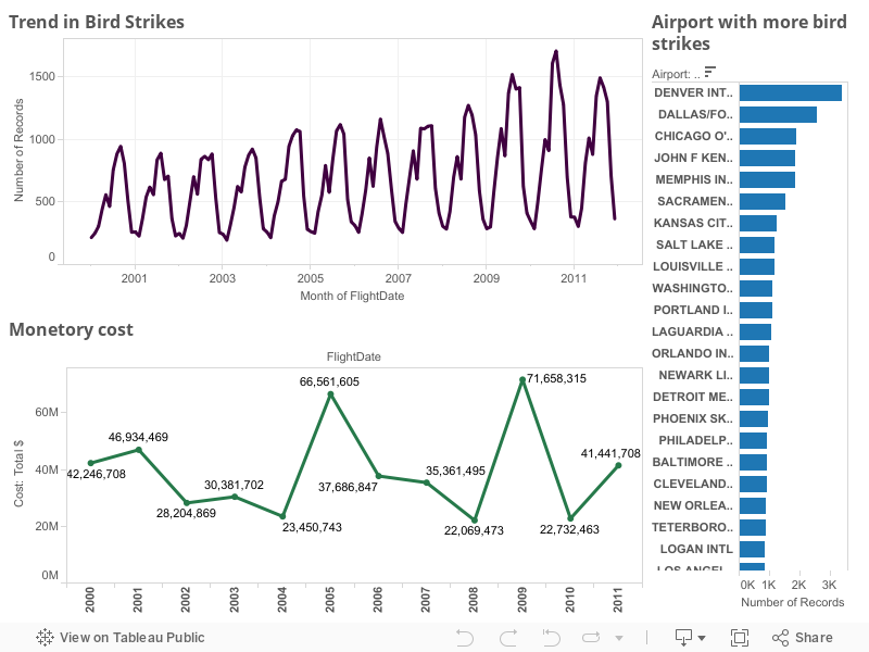
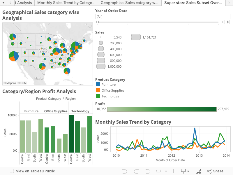
Superstore Sales Subset Overview
Olympic Medals Overview Globalwide
Interview Questions and Answers for TABLEAU
Advanced Tableau analysis
Advanced Analysis
Actions
Filter Actions
Highlight Actions
Selecting Marks to Highlight
Color Legend Highlighting
Highlight Toolbar Button
Creating Advanced Highlight Actions
URL Actions
Running Actions
Actions and Dashboards
Example: Filter Actions in a Dashboard
Example: URL Actions in a Dashboard
Using Field and Filter Values in Actions
Using Field and Filter Values in URLs
Using Field and Filter Values in Action Names
Calculations
Aggregations
How Aggregation and Disaggregation Work
Aggregating Data
Disaggregating Data
Example – Aggregating and Disaggregating Data
Calculated Fields
How to Create a Calculated Field
Copying and Pasting Calculated Fields
Writing formulas in Tableau
Example – Creating a Calculated Field
Aggregate Calculations
About Aggregate Calculations
How to Create an Aggregate Calculation
Aggregate Calculations in a Disaggregated State
Example – Aggregate Calculation
Example – Spotlighting Using Calculations
Table Calculations
Understanding Table Calculations
Addressing and Partitioning
Quick Table Calculations
Defining Basic Table Calculations
Difference From Calculation
Percent Difference From Calculation
Percent From Calculation
Percent of Total Calculation
Running Total Calculation
Moving Calculation
Secondary Table Calculations
Customizing Table Calculations
Binned Data
Example – Creating a Histogram with Binned Data
Totals
Grand Totals
How to Turn on Grand Totals
Grand Totals and Aggregations
Example – Grand Totals and Aggregations
Subtotals
Percentages
About Percentages
Percentages and Aggregations
Example – Percentages and Aggregations
Percentage Options
Percent of Table
Percent of Column
Percent of Row
Percent of Pane
Percent of Row in Pane
Percent of Column in Pane
Parameters
Creating Parameters
Editing Parameters
Using Parameters in Calculations
Parameter Controls
Example – Parameters
Background Images
Adding Background Images
Setting up the View
Managing Background Images
Editing an Image
Enabling/Disabling Images
Adding Show/Hide Conditions
Removing an Image
Background Maps
Geographic Roles
Building a Map View
Map Options
Map Layers
Data Layers
Washout
Setting a Default Location
Editing Locations
Custom Geocoding
Creating an Import File
Extending an Existing Role
Adding New Roles
Adding New Hierarchies
Importing Custom Geocoding
Saving Custom Geocoding
Background Map Sources
Working with WMS Servers
Setting a Default Map Source
Map Storing and Working Offline
Trend Lines and Statistics
Adding Trend Lines
Add Trend Lines to the View
Why can’t I add Trend Lines?
Remove Trend Lines
The Trend Line Model
Removing Factors from the Model
Testing Significance
Entire Model Significance
Significance of Specific Fields
Significance of Individual Trend Lines
Trend Lines Example
Assumptions
Trend Line Model Terms
Model Formula
Number of Observations
Residual DF (residual degrees of freedom)
DF (degrees of freedom)
SSE (sum squared error)
MSE (mean squared error)
R-Squared
Standard error
P (significance)
Analysis of Variance
Individual trend lines
Commonly Asked Questions
Log Axes
Advanced Analysis
Now that you understand the basics of building views in Tableau, become an advanced user by learning how to create custom calculations, use the built in statistics tools, leverage dynamic paramters, map data, and more.
• Actions
• Calculations
• Parameters
• Background Images
• Background Maps
• Trend Lines and Statistics
• Log Axes
Actions
Tableau allows you to add context and interactivity to your data using actions. Link to web pages, files, and other Tableau worksheets directly from your analytical results. Use the data in one view to filter data in another as you create guided analytical stories. Finally, call attention to specific results using highlighting.
For example, in a dashboard showing home sales by neighborhood you could use actions to help you quickly see relevant information for a selected neighborhood. Select a neighborhood in one view which then highlights the related houses in a map view, filters a list of the houses sold, and opens a webpage showing census data for the neighborhood.
There are three kinds of actions in Tableau: Filter, Highlight, and URL actions. This section discusses the following topics:
• Filter Actions
• Highlight Actions
• URL Actions
• Running Actions
• Actions and Dashboards
• Using Field and Filter Values in Actions
Filter Actions
Filter actions are a way to send information between worksheets. Typically a filter action is used to send information from a selected mark to another sheet showing related information. For example, when looking at a view showing the sales price of houses, you may want to be able to select a particular house and show all comparable houses in a different view. You could define a filter actions to accomplish this task. First you need to decide what comparable means. In this case, say that comparable houses are houses with a similar sale price and square footage. A filter action to show comparable houses can be defined by selecting a destination worksheet and defining filters on sales price and square footage.
Filter actions work by sending the data values of the relevant source fields as filters to the destination sheet. If you launch the filter action described in this example from a house that sold for $450,000, the destination sheet will have a filter to only show houses that sold for the same amount.
To create a filter action:
1. Select Edit > Actions.
2. In the Actions dialog box, click Add Action and then select Filter.
3. In the subsequent dialog box specify a name for the Action.
Use a name that defines the action. If you choose to run the action using the menu the name is the option that shows on the menu. For example, when sending housing information from one sheet to a map, the name could be “Map all comparable houses sold in February” You can use variables in the name that will be filled in based on the values of the selected field.
4. Use the drop-down list to select a source sheet or data source. When you select a data source or dashboard sheet you can further refine by selecting the individual sheets you want to launch the action from.
5. Then select how you want to launch the action. Select one of the following options:
o Hover – rest the pointer over a mark in the view to run the action. This option works well for highlight and filter actions within a dashboard.
o Select – click on a mark in the view to run the action. This option works well for all types of actions.
o Menu – right-click a selected mark in the view and then select an option on a the context menu. This option works well for filter and URL actions.
6. Use the second drop-down list to select a target sheet. When you select a dashboard sheet you can further refine the target by selecting one or more sheets within the dashboard.
7. Specify what do do when the select is cleared in the view. You can select from the following options:
o Leave the filter – leaves the filter on the target sheets. The target views in the dashboard will show the filtered results.
o Show all values – changes the filter to include all values.
o Exclude all values – changes the filter to exclude all values. This option is useful when you are building dashboards that only show some sheets if a value in another sheet is selected.
8. Setup one or more filters to specify the data that you want to show on the target sheets. You can filter on All Fields or define filters on Selected Fields.
9. If you are defining filters for specific fields click Add Filter.
10. In the Add Filter dialog box select a source and target data sources and fields. When you run the action from a specific mark on the source sheet, a filter is added to the target sheet that only includes values for the target field that match the values of the source field. In the comparable houses sheet link example, the Source Field is Beds and the Target Field is Beds. That means when you launch the sheet link for a house that has 3 bedrooms, the destination worksheet will only show houses that also have 3 bedrooms.
11. When finished, click OK three times to close the dialog boxes and return to the view.
You can add sheet links across data sources even if the field names are not exactly the same. One data source may have a field titled Latitude while another has a Lat field. Using the drop down lists in this dialog box, you can associate the Latitude field to the Lat field.
Note:
The fields available in the Target Field drop-down list are dependent on what you selected as the Source Field. Only fields with the same data type as the source field can be selected as a destination field.
Highlight Actions
Highlight actions allow you to call attention to marks of interest by coloring select marks and dimming all others. You can highlight marks in the view by selecting the marks you want to highlight, use the color legend to select related marks, or create an advanced highlight action.
• Selecting Marks to Highlight
• Color Legend Highlighting
• Highlight Toolbar Button
• Creating Advanced Highlight Actions
• Selecting Marks to Highlight
• When you select a mark in the view all other marks are dimmed to draw attention to the selection. Selection is saved with the workbook and can be included when publishing. The simplest way to add highlighting to a view is to select the marks you want to highlight.
• You can select multiple marks by holding down the Ctrl key on your keyboard while you select each mark. You can also click and drag the pointer to select all marks in a specific area of the view.
•
•
Color Legend Highlighting
Color legend highlighting is a powerful analytical mode for the color legend that allows you to focus on select members in the view. When you turn on color legend highlighting the marks associated with the selected items in the color legend are colored while all other marks are gray.
For example, the views below show the relationship between order quantity and profit for several products. The view on the left uses the normal color legend, all marks are colored based on their shipping mode. The view on the right uses legend highlighting to call out the products that were delivered via Delivery Truck.
You can easily switch between legend highlighting and normal modes using the color legend card menu. Then, if you like how a view is highlighted, you can assign the highlight colors to the color palette. The old colors are replaced with the highlight colors.
To turn on color legend highlighting:
1. Click the Highlight button at the top of the color legend or select Highlight Selected Items on the color legend card menu.
2. Select an item in the color legend.
Once legend highlighting is turned on, you can quickly focus on specific data in the view by selecting different items in the color legend. When color legend highlighting is turned on a Highlight Action is created and can be modified in the Actions dialog box.
To turn off color legend highlighting:
• Click the Highlight button at the top of the color legend or select Highlight Selected Items on the color legend card menu.
When you turn color legend highlighting off the action is removed from the Actions dialog box.
If you like how the view is highlighted and want to keep a specific member highlighted even when you turn off legend highlight mode, you can assign the highlight colors to the existing color palette. The original color legend is discarded and the highlight colors become the new color palette for the legend.
To assign the highlight colors to the color palette:
• Select Assign Highlight Colors to Palette on the color legend card menu.
Highlight Toolbar Button
Another way to add a highlight action is using the highlight button in the toolbar.Similar to the color legend highlighting, the toolbar button lets you highlight a collection of related marks in the view. To turn on highlighting, select the fields you want to use for highlighting on the toolbar menu. Then select a mark in the view to see the related data.
For example, the view below shows sales vs. profit by region. When a mark is selected, all other marks from that region that were shipped using the selected ship mode are highlighted. In this case you can quickly see all products from the Wester region that were shipped via Delivery truck.
The toolbar menu also lets you highlight on All fields or Dates & Times. All fields will consider all fields when determining matching records. Dates & Times considers all date and time fields.
When you use the Highlight toolbar button an action is created in the Actions dialog box. You can modify the action to create more advanced highlighting behavior.
Finally, you can use the toolbar button to disable highlighting across the entire workbook or for just the active sheet.
Creating Advanced Highlight Actions
You can define more advanced highlight actions using the Actions dialog. There you can specify source and target sheets along and the fields you want to use for highlighting. Follow the steps below to create a Highlight Action.
To create a highlight action:
1. Select Edit > Actions.
2. In the Actions dialog box click the Add Action button and then select Highlight.
3. Give the action a name that will identify it in the Actions dialog. Try to make it descriptive. For example, Highlight Products Shipped by Delivery Truck. You can use variables in the name that will be filled in based on the values of the selected field.
4. Use the drop-down list to select the Source sheet or data source. If you select a data source or a dashboard sheet you can further select individual sheets within them.
5. Select how you want to launch the action. You can select from the following options:
o Hover – rest the pointer over a mark in the view to run the action. This option works well for highlight and filter actions within a dashboard.
o Select – click on a mark in the view to run the action. This option works well for all types of actions.
o Menu – right-click a selected mark in the view and then select an option on a the context menu. This option works well for filter and URL actions.
6. Select a Target sheet. If you select a dashboard you can further select individual sheets within the dashboard.
7. Select the fields you want to use for highlighting. Select from the following options:
o Selected Fields – marks in the target sheet are highlighted based on select fields. For example, highlighting using the Ship Mode field will result in an action that highlights all marks in the target sheet that have the same ship mode as the selected mark in the source sheet.
o Dates and Times – marks in the target sheet are highlighted when their date and time match those of the marks selected in the source sheet. All dates and time fields are considered when determining a match.
o All Fields – marks in the target sheet are highlighted when they match the marks selected in the source sheet. All fields are considered when determining a match.
8. When finished, click OK twice to close the dialog boxes and return to the view.
URL Actions
A URL action is a hyperlink that points to a Web page, file, or other web-based resource outside of Tableau. You can use URL actions to link to more information about your data that may be hosted outside of your data source. To make the link relevant to your data, you can substitute field values of a selection into the URL as parameters.
To add a Hyperlink:
1. Select Edit > Actions.
2. In the Actions dialog box, click Add Action and then select URL.
3. In the subsequent dialog box, specify a name for the link. Make the name descriptive of the action. If you choose to run the action using the menu the name is the option that shows on the menu. For example, when linking to more product details, the name could be “Show More Details for Binder Clips.” You can use variables in the name that will be filled in based on the values of the selected field.
4. Use the drop-down list to select a source sheet or data source. If you select a data source or dashboard you can select individual sheets within it.
5. Select the fields you want to use for highlighting. Select from the following options:
o Hover – rest the pointer over a mark in the view to run the action. This option works well for highlight and filter actions within a dashboard.
o Select – click on a mark in the view to run the action. This option works well for all types of actions.
o Menu – right-click a selected mark in the view and then select an option on a the context menu. This option works well for filter and URL actions.
6. Specify the URL. You can use any URL that your browser can recognize including web pages, ftp resources, and files.
Just as you can use variables in the name of the URL, you can also use field values and filter values as parameters in the URL. That means that you can send information about each selected mark or filter setting to a given website.
7. Optionally select one or more of the following options:
o URL Encode Data Values – select this option if your data contains values that use characters that are not allowable in a URL. For example if one of your data values contains an ampersand, such as “Sales & Finance,” the ampersand must be translated into characters that your browser understands (URL encoded) if you want to include that value in the URL.
o Enable Multi-Select – select this option if you are linking to a webpage that can take lists of values as parameters in the link. For example, say you select several products in a view and you want to see each product’s details hosted on a webpage. If the server can load multiple product details based on a list of identifiers (product ID or product name), you could use multi-select to send the list of identifiers as parameters.
When you enable multi-select you must also define the item delimiter, which is the character that separates each item in the list (often a comma). You must also define the Delimiter Escape, which is used if the delimiter character is used in a data value.
8. When finished, click OK twice to close the dialog boxes and return to the view.
Note:
URL actions can also point to a web page object in a dashboard. Refer to Actions and Dashboards to learn more about how actions work with dashboards.
Running Actions
Depending on how the action is created you can run an action using one of the following three methods:
• Hover – rest the pointer over a mark in the view to run the action. This option works well for highlight and filter actions within a dashboard.
• Select – click on a mark in the view to run the action. This option works well for all types of actions.
• Menu – right-click a selected mark in the view and then select an option on a the context menu. This option works well for filter and URL actions.
Hover Select Menu
Links are not always visible for every worksheet and mark. Because links are mapped to specific fields in the data source, links will only be available for the worksheets that use the mapped fields. For example, if you add a hyperlink that uses both Latitude and Longitude as parameters in the link, the link will only be available to worksheets that use Latitude and Longitude in the view. Additionally, the link is only available on marks and headers that contain relevant values.
Actions and Dashboards
Actions often have special behavior when the source or destination is a dashboard. Filter and Highlight actions can affect other views in the dashboard and and URL actions can update a webpage object so you don’t have to open your web browser. Finally, you can create simple Filter and Highlight actions using special menu options so you don’t have to open the Actions dialog box.
• Example: Filter Actions in a Dashboard
• Example: URL Actions in a Dashboard
• Example: Filter Actions in a Dashboard
• This example shows how to create a filter action in a dashboard. The example shows a Real Estate dashboard with three views. Using the Use as Filter option you can set one of the views to act as a filter on all the other views in the dashboard. In this case the scatter plot in the upper right is filtering the map view and the text table to show more details about the selected houses.
•
•
•
• The Use as Filter command can only apply to one view at a time. A filter action is created that you can modify in the Actions dialog box.
Example: URL Actions in a Dashboard
This example shows how a URL action works with a web page object in a dashboard. Below is a dashboard showing sales information by product for several stores in a coffee franchise. Included in the dashboard is a web page object that shows product details. The text table has a URL action that points at that web page. When you launch the action the web page automatically updates within the dashboard rather than opening a web browser.
Using Field and Filter Values in Actions
When you add an action in Tableau you often want to use values from your data as parameters in the name of the action as well as the action itself. Using fields as variables in the action name makes the menu item that launches the action specific to the selected mark. More commonly, using field and filter values as parameters in the URL of a URL action allows you to send information about a specific data point or filter setting to the destination webpage.
• Using Field and Filter Values in URLs
• Using Field and Filter Values in Action Names
Using Field and Filter Values in Action Names
In addition to using field and filter values in URLs, you can use field and filter information as variables in the action names. The name of the action displays on the context menu when an action is launched using the menu. Using field and filter variables in the name is useful in making the action specific to the selected mark. In a view showing real estate information, you could name a URL action that points at satellite images from an online mapping service, “Show satellite image of <Address>.” When you right-click on a specific mark, the <Address> tag is replaced with the location value associated with that mark.
To add a field or filter as a variable in a Name:
1. In the Add Action dialog box, begin typing the name for the action.
2. Place the cursor where you want to insert the field or filter value.
3. Click the arrow to the right of the text box and select the field or filter you want to add as a variable. The field or filter name is added between angle brackets.
Calculations
To extract meaningful results from your data, you might want to perform one or more calculations. Some calculations are predefined in Tableau, while you can customize others to suit your specific needs. The following calculations are supported:
• Ag gre gations – View your data at different levels of detail. For example, you might want to view data in an aggregated state such as a summation or an average, or you might want to view the data in a disaggregated state and work with the individual rows of a data source.
• Calcula ted Fields– Create new fields that are based on existing data source fields, and common functions and operators. Use a standard dialog box that shows available functions and fields to author these custom fields.
• Table Calculations – Create calculations that are applied to the values in the entire table and are often dependent on the table structure itself, such as running totals and year to date growth.
• Bin ned Data – Create new fields that are based on binned measures.
• Su btot als – Add subtotals to the rows and columns of a table.
• Gr and Totals – Add totals to the rows and columns of a table.
• Pe rcent ages – View data as percentages rather than as absolute numbers. The percentages can be based on rows, columns, panes, or the entire table.
You can use all of these different types of calculations simultaneously. For example, you can create a new calculated field called Profit that is the difference between the Sales and Cost fields. You could then apply an aggregation (like a summation) to this new field in order to view total profit over time. You could then display the numbers as percentages and turn on grand totals to see how these percentages vary from category to category. Finally, you could bin the new field and display the data as a histogram.
• Aggregations
• Calculated Fields
• Table Calculations
• Binned Data
• Totals
• Percentages
Aggregations
Sometimes it is useful to look at numerical data in an aggregated form such as a summation or an average. The mathematical functions that produce aggregated data are called aggregation functions. Aggregation functions perform a calculation on a set of values and result in a single value. For example, a measure that contains the values 1, 2, 3, 3, 4 aggregated as a sum results in a single value: 13.
For example, if you have 3,000 sales transactions from 50 products in your data source, you might want to view the sum of sales for each product, so that you can decide which products are the most important.
Tableau provides a set of predefined aggregations that are shown in the table below.
Aggregation Description Result for measure that contains 1, 2, 2, 3
ATTR Returns the value of the given expression if it only has a single value for all rows in the group, otherwise it displays an asterisk (*) character. Null values are ignored. N/A
Dimension Returns all unique values in a measure or dimension. 3 values (1, 2, 3)
Sum Computes the sum of the numbers in a measure. Null values are ignored. 1 value (8)
Average Computes the arithmetic mean of the numbers in a measure. Null values are ignored. 1 value (2)
Minimum Computes the smallest number in a measure or continuous dimension. Null values are ignored. 1 value (1)
Maximum Computes the largest number in a measure or a continuous dimension. Null values are ignored. 1 value (3)
Standard Deviation Computes the standard deviation of all values in the given expression based on a sample population. Null values are ignored. Returns a Null if there are fewer than 2 members in the sample that are not Null. Use this function if your data represents a sample of the population. 1 value (0.8165)
Standard Deviation Population Computes the standard deviation of all values in the given expression based on a biased population. Assumes that its arguments consist of the entire population. Use this function for large sample sizes. 1 value (0.7071)
Variance Computes the variance of all values in the given expression based on a sample. Null values are ignored. Returns a Null if there are fewer than 2 members in the sample that are not Null. Use this function if your data represents a sample of the population. 1 value (0.6667)
Variance Population Computes the variance of all values in the given expression based on a biased population. Assumes that its arguments consist of the entire population. Use this function for large sample sizes. 1 value (0.5000)
Count Counts the number of rows in a measure or a dimension. When applied to a dimension, Tableau creates a new temporary column that is a measure because the result of a COUNT is a number. You can count numbers, dates, booleans, and strings. Null values are ignored in all cases. 1 value (4)
Count Distinct Counts the number of unique values in a measure or dimension. When applied to a dimension, Tableau creates a new temporary column that is a measure because the result of a COUNT is a number. You can count numbers, dates, booleans and strings. Null values are ignored in all cases. This function is not supported for Microsoft Access, Microsoft Excel, and Text file data sources. 1 value (3)
Disaggregate Returns all records in the underlying data source. 4 values (1, 2, 2, 3)
You can also define custom aggregations as described in Aggre gate Calculations. Note that depending on the type of data view you create, Tableau will apply these aggregations at the appropriate level of detail. For example, Tableau will apply the aggregation to individual dimension members (the average delivery time in the East region), all members in a given dimension (the average delivery time in the East, West, and Central regions), or groups of dimensions (the sum of sales for all regions and for all markets).
You may specify a default aggregation for any measure that is not a user-defined aggregation. A default aggregation is a preferred calculation for summarizing a continuous or discrete field. The default aggregation is automatically used when a measure is first placed on a shelf. Change the default aggregation by right-clicking a measure in the Data window and selecting Field Properties > Aggregation. Below the default aggregation for the Budget Margin measure is set to Average.
Tableau also allows you to view data in disaggregated form (relational databases only). This is an extremely powerful feature. When data are disaggregated, you can view all of the individual rows of your data source. For example, after discovering that the sum of sales for rubber bands is $14,600, you might want to see the distribution of individual sales transactions. To answer this question, you need to create a view that shows individual rows of data. That is, you need to disaggregate the data (refer to How Agg regatio n and Disaggregation Work). Also, one way to look at disaggregated data is to view the underlying data that’s displayed in a table.
• How Aggregation and Disaggregation Work
How Aggregation and Disaggregation Work
When you place a measure on a shelf, Tableau automatically aggregates the data, usually by summing it. You can easily determine the aggregation applied to a field because the function always appears in front of the field’s name when it is placed on a shelf. For example, Profit becomes SUM(Profit).
This section discusses the following topics:
• Aggregating Data
• Disaggregating Data
• Exa mple – Aggregating a nd Disaggregating Data
• Aggregating Data
• Disaggregating Data
• Example – Aggregating and Disaggregating Data
Aggregating Data
You can change the aggregation of a field by selecting a different function from the field’s context menu. As shown below, all of the predefined aggregations are available from this menu.
Aggregating Measures
You can assign a different aggregation to every measure you place on a shelf. For example, you can aggregate Salesas a summation, Profit as a maximum, and Discount as an average.
You can change the aggregation state for all the measures on a worksheet by selecting the Analysis > Aggregate Measures menu item.
When all measures are disaggregated you see a mark for each row in the view. You cannot select specific marks to Keep Only, Exclude, or create a Set when all measures are disaggregated.
Aggregating Dimensions
When you aggregate dimensions, you create a new temporary measure column, so the dimension is now viewed as a measure. While you cannot apply all of the other predefined aggregations to a dimension, you can apply Dimension, Minimum, Maximum, and Count.
Disaggregating Data
Disaggregating your data allows you to view every row of the data source which can be useful when you are analyzing measures that you may want to use both independently and dependently in the view. For example, you may be analyzing the results from a product satisfaction survey with the Age of participants along one axis. You can aggregate the Age field to determine the average age of participants or disaggregate the data to determine at what age participants were most satisfied with the product.
You can disaggregate all measures in the view by selecting Analysis > Aggregate Measures.
Example – Aggregating and Disaggregating Data
This example includes several views of aggregated and disaggregated data created using the Sample – Superstore Sales data source. To create the views, follow these five steps:
1. Place the Sales measure on the Columns shelf and the Profit measure on the Rows shelf.
The measures are automatically aggregated as sums. The aggregation is indicated by the field names and by the tooltip. The values shown in the tooltip are the sales and the profit for the entire data source. That is, the summations are performed using every row in the data source.
2. Place the Product 1 – Category dimension on the Color shelf.
One way to show more data in your view is to disaggregate the measures. Another way is to show additional levels of detail. For example, placing the Product 1- Category dimension on the Color shelf separates the data into three marks—one for each dimension member—and then encodes the marks using color.
Although more marks are displayed, the measures are still aggregated. The single mark in the view indicates the sum of the sales and the sum of the profit for Office Supplies. If you were to sum the sales and profit values for the three marks, you would produce the values for the entire data set as given in the previous step of this example.
3. Place the Discount measure on the Filters shelf.
In the Filter Field dialog box select All Values to filter on the disaggregated measure.
Filter the data to only include discounts greater than 6% (0.06). Because Discount is disaggregated, Tableau applies the filter to each row in the data source before performing the aggregations for the Sales and Profitmeasures.
The view is shown below. The tooltip indicates that both the sales and the profit numbers are smaller than in the previous view. This is because data have been filtered out of the aggregation operation.
4. Change the aggregation of Sales to an average.
The measures are not required to have the same aggregation. Change the aggregation by selecting Averagefrom the field’s context menu.
The view is shown below. The field name and tooltips indicate the new aggregation.
5. Disaggregate the data.
All measures—except those placed on the Filters shelf—must have the same aggregation state. That is, they must all be either aggregated or disaggregated.
You change the aggregation state by selecting the Analysis > Aggregate Measures menu item.
The view is shown below. Disaggregating the data displays every row in the data source that passes through the filter. The tooltip shows the profit and sales for one particular row.
Calculated Fields
You might find that your data source doesn’t include all of the fields needed to answer your questions. For example, you might want to create a new calculated field called Profit that is the difference between the Sales and the Cost fields, or you might want to create a conditional statement that divides the Sales Budget field into values that are under budget and values that are over budget.
Tableau allows you to create a new calculated field by defining a formula that is based on data source fields and other calculated fields, and that uses standard functions and operators.
• How to Create a Calculated Field
• Copying and Pasting Calculated Fields
• Writing formulas in Tableau
• Example – Creating a Calculated Field
• Aggregate Calculations
• Example – Spotlighting Using Calculations
How to Create a Calculated Field
To create a new calculated field, select Analysis > Create Calculated Field, or select Create Calculated Field on one of the Data window title menu.
The Calculated Field dialog box opens.
To define the calculation do the following:
1. Specify a name for the new field.
2. Create a formula that defines the new field. Refer to Writing for mulas in Tableau for more information about how to define a formula.
3. When finished, click OK.
The new calculated field displays in either the Dimensions area or the Measures area of the Data window depending on the data type returned by the calculation. Calculations that return a string or date are dimensions, while calculations that return a number are measures. In the latter case, you can convert the measure to a dimension if you want to treat the calculated values as discrete rather than continuous.
Copying and Pasting Calculated Fields
Calculated fields are available to all sheets that use the same data source in a single workbook. In addition, you can copy and paste these custom fields between workbooks simply by right-clicking the field in the Data window and selectingCopy. Then in the new workbook, right-click the Data window and select Paste. You can copy and paste all custom defined fields such as calculated fields, ad-hoc groups, user filters, sets, and so on.
Writing formulas in Tableau
The formula editor has built-in coloring and validation to help you avoid syntax errors. As you write the formula, syntax errors are underlined with a red squiggly line. Hover over the error to see directions for fixing it. Also any errors with the caluclation are shown in a drop-down list. When the cacluation is valid, a green check mark is displayed.
When you are writing formulas, any part that displays in bold indicates that it will be computed locally within Tableau on the aggregated results. Any normal weight text will be computed at the database level.
Formuals are made up of the following parts:
1. Functions
The Functions area of the dialog box contains all the functions you can use to create a formula. The functions are organized into categories, which are available from the drop-down menu. By default all functions are displayed.
You can display a brief description for each function by clicking its name in the list box. Double-click a function to include it in a formula. Functions are colored black in the formula.
2. Fields
All data source fields and calculated fields are listed in the Fields area of the dialog box. Binned fields and setsare not listed because they cannot be used in calculations.
The field’s data type and the name display in the list. Use the drop-down menu to select a secondary data source and see its fields.
Double-click a field name to include it in a formula. You can also just type the bare field name. However, if the field name includes special characters such as spaces, it must be delimited with square brackets as inSUM([Store Profit]). A right bracket (]) can be doubled to include it in the field name itself. For example, the field name “Store Profit]” would be written as [Store Profit]]].
Fields are colored orange in the formula.
3. Operators
Operators are not available on the dialog box like functions and fields. Instead, you must manually type the operators into your formula. All standard operators such as addition (+), subtraction (–), multiplication (*), and division (/) are supported. Operators are colored black in the formula.
4. Parameters (optional)
Parameters are placeholders variables that can be inserted into calculations to replace constant values. When a parameter is used in a calculation, you can then use a parameter control to dynamically change the value. Parameters are colored purple in the formula.
5. Comments (optional)
You can insert custom comments for your calculations as a means of annotation for later review. To add a comment to a calculation type two forward slash characters into the formula pane.
For example:
Sales * Profit //John’s calculation
In this example //John’s calculation is a comment.
A comment starts at the two forward slashes (//) and goes to the end of the line. A multiline comment can be written by starting each line with two forward slashes (//). Comments are colored green in the formula.
Example – Creating a Calculated Field
In this example we will create a calculated field using Tableau formulas and use the new field in a data view. Then we’ll edit the field’s formula to create a new view, and finally delete the field from the Data window. This example uses the Sample – Superstore Sales (Excel) data source.
1. Create the view.
Select New Calculated Field on the Data window menu.
2. Complete the Calculation dialog box.
Name the new field Discount Ratio and enter the formula shown below.
IIF([Sales] !=0, [Disocunt]/[Sales],0)
You can type the formula by double clicking the field names in the Fields list and functions in the Functions list. You must type the operators (!= and /) manually. Note that the IIF statement is used to avoid dividing by zero.
The new field displays in the Measures area of the Data window because the calculation returns a number. You can use this new field just like any other field.
3. Add the calculation to the view.
Place Ship Mode on the columns shelf, Region on the Rows shelf, and Product 1- Category on the Color shelf. Then place the new calculation, Discount Ratio onto the Rows shelf. Note that you can treat the new calculation just like any other measure. For example, you can apply an aggregation to it. Below, Discount Ratio is aggregated as a maximum.
4. Edit the calculation.
You can change the field’s formula by right-clicking the field name in the Data window and selecting Edit or by selecting Analysis > Edit Calculation.
In the Calculated Field dialog box, change Sales to Order Quantity.
The view automatically updates after you click OK in the Calculated Field dialog box.
5. Delete the calculated field.
You can delete a calculated field by right-clicking the field name in the Data window and selecting Delete fromthe right-click context menu. Before deleting the field, you might want to save your workbook. If you do not save your work, the calculated fields will be lost.
Aggregate Calculations
Aggregate functions allow you to summarize data. As described in Ag gre gations, Tableau includes a variety of predefined aggregations such as summation and variance. An aggregate calculation allows you to define aggregations other than these predefined choices.
• About Aggregate Calculations
• How to Create an Aggregate Calculation
• Aggregate Calculations in a Disaggregated State
• Example – Aggregate Calculation
About Aggregate Calculations
Suppose you want to analyze the overall gross margin for every product in your data source. One way to do this is to create a new calculated field called Margin that is equal to the profit divided by the sales. Then you could place this measure on a shelf and use the predefined summation aggregation. In this scenario, Margin is defined as follows:Margin = SUM([Profit]/ [Sales])
This formula calculates the ratio of profit and sales for every row in the data source, and then sums the numbers. That is, the division is performed before the aggregation. However, this is almost certainly not what you would have intended because summing ratios is generally not useful.
Instead, you probably want to know the sum of all profits divided by the sum of all sales. That formula is shown below.
Margin = SUM( [Profit]) / SUM([Sales])
In this case, the division is performed after each measure is aggregated. An aggregate calculation allows you to create formulas like this.
How to Create an Aggregate Calculation
When a calculation uses an aggregate function, it’s called an aggregate calculation. You create an aggregate calculation by defining a new calculated field as described in Ho w to Create a Ca lculated Field. The formula will contain one or more aggregate functions. You can easily pick an aggregate function from the Calculation dialog box by selecting Aggregate from the Functions menu as shown below.
These functions are identical to the predefined aggregate functions listed in Ag gre gations.
The aggregate calculation appears with the letters AGG in front of it when it is placed on a shelf.
When you create an aggregate calculation, no further aggregation of the calculation is possible. Therefore, the field’s context menu does not offer any aggregation choices. However, you can disaggregate the field. Refer to Agg regate Calculati ons in a Disaggregated State for more information.
The rules that apply to aggregate calculations are:
• For any aggregate calculation, you cannot combine an aggregated value and a disaggregated value. For example, SUM(Price)*[Items] is not a valid expression because SUM(Price) is aggregated and Items is not. However, SUM(Price*Items) and SUM(Price)*SUM(Items) are both valid.
• Constant terms in an expression act as aggregated or disaggregated values as appropriate. For example:SUM(Price*7) and SUM(Price)*7 are both valid expressions.
• All of the functions can be evaluated on aggregated values. However, the arguments to any given function must either all be aggregated or all disaggregated. For example: MAX(SUM(Sales),Profit) is not a valid expression because Sales is aggregated and Profit is not. However, MAX(SUM(Sales),SUM(Profit))is a valid expression.
• An aggregate calculation is always a measure.
• Like predefined aggregations, aggregate calculations are computed correctly for grand totals. Refer to Gr and To tals and Aggregations for more information.
• ggregate Calculations in a Disaggregated State
• If an aggregate calculation is disaggregated, the calculation is modified in a way that depends on the functions used. Every function has a disaggregated substitute, as shown below.
Aggregation Function Disaggregated Substitute
AVG(data) data
COUNT(data) IIF(ISNULL(data),0,1)
COUNTD(data) IIF(ISNULL(data),0,1)
MAX(data) data
MIN(data) data
STDEV(data) Null
STDEVP (data) IIF (ISNULL (data), Null, 0)
SUM(data) data
VAR(data) Null
VARP (data) IIF (ISNULL (data), Null, 0)
• Note that STDEV and VAR are Nullbecause those functions return Null if there are fewer than two elements in a group that are not Null, and each group has size 1 when it is disaggregated. Refer to Ag gre gations for descriptions of the aggregation functions.
• Therefore, if you define an aggregate calculation called Margin that is equal to SUM(Profit)/SUM(Sales) and then disaggregate the data, it is interpreted as Profit/Sales.
Example – Aggregate Calculation
In this example you will use the Sample – Superstore Sales data source to create an aggregate calculation called Margin, and use the new field in a data view.
1. Select New Calculated Field on the Data window menu.
2. Define the calculation.
Name the new field Margin and enter the formula shown below.
IIF(SUM([Sales]) !=0, SUM([Profit])/SUM([Sales]), 0)
You enter the formula by selecting functions from the Functions area of the dialog box, and field names from theFields area of the dialog box. You must type the operators (!= and /) manually. Note that the IIF statement is used to avoid dividing by zero.
The new calculated field displays in the Measures area of the Data window where you can use it like any other measure.
A view using the new aggregate measure is shown below.
When Margin is placed on a shelf, its name is automatically changed to AGG(Margin), which indicates it’s an aggregate calculation. Additionally, the field’s context menu does not include any aggregation choices because aggregating a field that’s already aggregated is not possible.
Example – Spotlighting Using Calculations
Spotlighting is a term that applies a calculation that shows discrete thresholds based on the values of a measure. For instance, you might want to color-code sales so that those over 10,000 appear green and those below 10,000 appear red.A spotlighting calculation is just a special case of a calculation that results in a discrete measure. A discrete measure is a calculation that is a dependent variable (and therefore a measure), but which results in a discrete result (as opposed to a continuous result). Thus the name discrete measure. Here is an example:
The formula in this example defines a discrete measure called “Sales Spotlight.” Discrete measures always appear with a blue “abc” icon in the Data window. The example above is a measure because it is a function of another measure. It’s discrete because it produces discrete values (“Good” and “Bad”) as a result rather than continuous values like numbers. Here is an example of this categorical measure in use:
Here the “sales spotlight” field is on the Color Shelf. It appears with the “AGG” prefix because it is an aggregate calculation. Values above 10,000 and below 10,000 are assigned different colors. This type of discrete highlighting is often called spotlighting.
Table Calculations
Another kind of calculation is a table calculation. Table Calculations are computations that are applied to the values in the entire table and are often dependent on the table structure itself. For example, in a sales environment, you can use table calculations to compute the running total of sales across a specified date range or to compare multiple months of sales and compute each month’s contribution to the total sales.
All table calculations are computed locally using the values you see in the table. This means that computing a moving average for a measure that is aggregated as an average results in an average of the averages.
You can add table calculations to your view using either the predefined quick calculations or by specifying a custom definition.
• Understanding Table Calculations
• Quick Table Calculations
• Defining Basic Table Calculations
• Secondary Table Calculations
• Customizing Table Calculations
Understanding Table Calculations
Table calculations are computations that are applied to the values in the table. These computations are unique in that they usse data from multiple rows in the database to calculate a value. To create a table calculation, you need to define both what you want to compute and what to compute along. For example, when defining a running sum calculation for several years you are computing a running sum along the Date field. These are defined in the calculated field dialog box using the Calculation Type and Calculate Along drop-down menus.
The definition of what to compute along has two parts: addressing fields and partitioning fields.
• Addressing and Partitioning
Addressing and Partitioning
The addressing fields define what part of the table you are computing along. The partitioning fields define how to group the calculation. In the example of a running sum of product sales across several years, the addressing field is the Date field while the parititioning field is the product field. When youd define the addressing for a table calculation, all the other fields are used for partitioning.
You can specify the addressing in the Table Calculation dialog box. The addressing can be relative to the table structure or a specific field. Each addressing option is described below.
Table (Across)
This option sets the adressing to compute along the entire table moving horizontally through each partition. For example, the view below shows quarterly sales by region and product category. When a calculation addressing is set to Table Across, the fields that span horizontally across the table are the addressing fields (Category and Region). All the other fields (Year, Quarter) are partitioning. The addressing fields are shown in orange while partitioning fields are shown in blue.
That means that each partition will be the combination of Year and Quarter.
Table (Down)
This option sets the addressing to compute along the entire table moving vertically through each partition. For example, the same view from above is shown below with the addressing set to compute along Table Down. The fields that span vertically (Year, Quarter) are now the addressing fields and the rest of the fields are partitioning (Category and Region). The addressing fields are shown in orange while partitioning fields are shown in blue.
That means that each partition is the combination of Category and Region.
Table (Across then Down)
This option sets the addressing to compute across the entire table horizontally and then down the table vertically. This means that both the fields that span across the table and down the table are addressing fields.
That means that the entire table is the partition. The computation will compute across, move to the next row and continue to compute across, and so on.
Pane (Across)
This option sets to compute across the pane horizontally. The fields that span across the pane horizontally are the addressing fields. However, the fields that separate the panes are now partitioning fields. In the example below Category becomes a partitioning field along with Year and Quarter. Region is the addressing field.
That means that the combination of Year, Quarter, and Category is the partition.
Pane (Down)
This option sets the addressing to compute down the table within the pane. The fields that separate the pane (Category and Year) are partitioning fields. In addition, the Region field becomes a partitioning field while the Quarter field is the addressing field.
That means that the combination of Year, Category, and Region is the partition.
Pane (Across then Down)
This option sets the addressing to compute across within the pane, then move to the next row and continue to compute across. The addresssing fields are both the fields that run across the table horizontally and down the table vertically (Region and Quarter). The partitioning fields are the fields that define the pane (Category and Year).
That means that the combination of Category and Year make up the partition.
Cell
This option sets the addressing to the indvidual cells in the table. All fields become partitioning fields. This option is generally most useful when computing a percent of total calculation.
That means that the partition is the combination of Category, Region, Year, and Quarter.
Individual Fields
This option sets the addressing to compute across the field you specify. The benefit of this option is that you get absolute control over how the calculation will be computed. Be careful though, because, addressing on an individual field means that when you rearrange the table, the calculation may no longer match the table structure.
Advanced
The advanced option lets you specify multiple fields to act as the addressing fields. When you select Advanced another dialog box opens where you can specify one or more fields to act as addressing fields. Then you can specify how to order those fields.
For example, in the view below the addressing fields are set to Category and Year. These are ordered by SUM(Sales) Descending. That means that the combination of Quarter and Region create the partition. Q1 Central exists four times in the table, and that is the partition.
Because the order is set to SUM(Sales), the calculation is computed based on their SUM(Sales) values from highest to lowest.
Quick Table Calculations
You can add common table calculations to your view using the Quick Table Calculations menu item on the field context menus. These quick calculations are predefined table calculations based on the most common scenarios.
To add a quick table calculation:
1. Right-click the measure you want to use in the table calculation and select Quick Table Calculation.
2. On the sub-menu select one of the following options:
o Running Total
o Difference
o Percent Difference
o Percent of Total
o Moving Average
o Year to Date (YTD) Total
o Compound Growth Rate (CAGR)
o Year over Year Growth
o Year to Date (YTD) Growth
After adding the quick table calculation to the view, you can edit the definition by selecting Edit Table Calculation on the field’s context menu
efining Basic Table Calculations
When you add a Table Calculation to the view, you need to specify the parameters that define the formula used in the computation. All of these parameters are set in the Table Calculation dialog box.
To manually define a table calculation:
1. Right-click the measure you want to use in the computation and select Add Table Calculation.
2. In the Table Calculation dialog box, select one of the following types of calculations from the drop-down menu at the top:
o Differ ence From Calculation – compute the difference between two specified values.
o Percent Differe nce From Calculation – compute the difference between two specified values as a percentage.
o Percent From Calc ulation -compute each value as a percentage of another specified value.
o Percent of Total Cal culation – compute each value as a percentage of the total measure.
o Runn ing Total Calculation- compute cumulative totals along a specified dimension.
o Movi ng Calculation – summarize a range of values using the specified aggregation to smooth short fluctuations and reveal long term trends.
3. Define the formula using the drop-down lists in the bottom half of the dialog box. Learn more about how to define each type of calculation by selecting it in the list above.
4. When finished click OK. The measure is now marked as a table calculation and all the relevant values in the view are computed using the table calculation.
• Difference From Calculation
• Percent Difference From Calculation
• Percent From Calculation
• Percent of Total Calculation
• Running Total Calculation
• Moving Calculation
• Difference From Calculation
• Use this type of calculation to compute the difference between two specified values in the table along a certain dimension. For example, compute the difference between 2006 and 2007 quarterly sales for four different customer segments.
• When defining a Difference From calculation, you need to specify a dimension or table structure to compute across, the dimension level to use in the computation (this is only required if you are computing across a dimension), and a value to compare the current value to. The following is an example of a Difference From calculation.
• Example: Difference From Calculation
• The table below shows the 2006 and 2007 quarterly sales numbers for several different customer segments of a superstore.
•
•
•
• To compute the difference between 2008 and 2009 sales, you can define a table calculation using the definition shown below.
•
•
•
• The difference is calculated along the Order Date dimension at the level of year because we are comparing 2008 sales to 2009 sales. The table now displays the difference between each quarter in 2009 and the corresponding quarter in the previous year. Notice that there are no values for 2008. That’s because there are no previous years to compute the difference from. You can hide that column without affecting the calculation.
•
•
•
• The view below may be more clear. It shows both the Difference From calculation and the Total Sales (before the computation). You can see that in the first quarter of 2009 the total sales was $203,761 while in the same quarter in 2008 the total sales was $191,307. The difference between these two values is $12,454.
•
•
•
• Note:
• You can add a Difference From calculation to your view quickly by right-clicking the measure you want to use in the computation and selecting Quick Table Calculations > Difference. This quick calculation computes the difference between values across rows where each difference is calculated against the previous value. Refer to Quick Ta ble Calc ula tions.
• Percent Difference From Calculation
• Use this type of calculation to display the rate of change between two specified values in the table by computing the difference as a percentage. A common use of this type of calculation is to compute the percent gain year after year (CAGR).
• Similar to the Difference From calculation, to define a Percent Difference From calculation you need to specify a dimension or table structure to compute across, the dimension level to use in the computation (this is only required if you are computing across a dimension), and a value to compare the current value to. The following is an example of a Percent Difference calculation.
• Example: Percent Difference From Calculation
• The table below shows the profit for several customer segments over four years. Looking at the view, we can see that there was a drop in profit in the Small Business and Consumer segments in 2007.
•
•
•
• When we view this same view using a Percent Difference From calculation, it becomes clear that Small Business segment rebounded quite dramatically in 2008.
•
•
•
• You can define a Percent Difference From calculation like this using the table calculation definition shown below.
•
•
•
• The difference is calculated along the Order Date dimension at the Year level because we are comparing year after year profit. Each value in the view is a difference of the previous year. The view below shows each year as a difference of 2006 Profit. You can see that the Corporate segment is the only one to be above the 2006 profits in 2009.
•
•
•
• Note:
• Percent Difference From calculations are commonly used to calculate compound growth rates and year over year growth. You can quickly add these calculations by right-clicking the measure you want to use in the calculation and selecting the calculation on the Quick Table Calculation sub-menu. Refer to Quick Ta ble Calc ula tions.
• Percent of Total Calculation
• Use the Percent of Total calculation to compute the percentage a specified value contributes to the total. For example, you can use this type of calculation to view the contribution each member in a sales team makes to the total company sales each quarter.
• For a Percent of Total calculation you must specify a dimension or table structure to compute across and the dimension level to use in the computation. The dimension level is only necessary if you have chosen to compute across a dimension rather than a table structure. The following is an example of a Percent of Total calculation.
• Example: Percent of Total Calculation
• In this example, imagine that we are analyzing the performance of several stores. The view below shows the sales performance for three different regions. From the view we can see that the Southern region (orange marks) has the highest sales.
•
•
•
• When we add the Percent of Total table calculation to the view, we can see that the South region accounts for just over 27% of the total sales.
•
•
•
• The table calculation was computed using the definition shown below. The total was computed across each row in the table.
•
•
•
• Note:
• You can add a Percent of Total calculation quickly to your view by right-clicking the measure you want to use in the computation and selecting Percent Total on the Quick Table Calculations sub-menu. Refer to Quick Ta ble Calc ula tions.
Running Total Calculation
Use the Running Total calculation to compute a cumulative total across a dimension or table structure. For example, you can use this type of calculation to calculate the cumulative sales for each quarter for several years.
When you define a running total calculation, you need to specify an aggregation to use when summarizing the values. For example, the most common aggregation will be sum so you can see the summation of values, but sometimes you may want to use average or another aggregation. You also need to specify the dimension to compute a running total across. This can either be an actual dimension in the data source or a table structure like rows or columns. Finally, you need to specify when to restart the at zero and begin totaling again. The following is an example of a Running Total calculation.
Example – Running Total Calculation
The view below shows the total quarterly sales from 2006 to 2009.
While it is useful to see each quarter’s sales, you may also want to see the cumulative totals for each quarter in the year. To create this kind of view we can add a Running Total calculation. The view below shows the running totals for each quarter restarting at zero for each year. That means that the Quarter 4 shows the total sales for that year.
This calculation was defined by the formula shown below. We are summarizing values as a sum along the Order Date dimension restarting at zero every Year.
Note:
You can add a Running Total calculation to your view easily using the Quick Table Calculations menu. Right-click the measure you want to use in the calculation and select Quick Table Calculations > Running Total. Refer to Quick Ta ble Calc ula tions.
Moving Calculation
A moving calculation is typically used to smooth short term fluctuations in your data so that you can see long term trends. A good example is when you are looking at securities data. There are so many fluctuations every day that it is hard to see the big picture through the daily ups and downs. You can use a moving calculation to define a range of values to summarize using an aggregation of your choice.
When you define a moving calculation you must first specify the aggregation you want to use when summarizing that data. The most common aggregation for this type of calculation is an average. Next you need to specify the dimension to summarize across. You can select a table structure such as Rows or Columns or an actual field in your data source. Once you have selected a dimension, define the number of values before the current value and the number of values after the current value to include in the summary. You can also decide whether to include the current value using the checkbox on the right. The following is an example of a Moving Calculation.
Example – Moving Calculation
The view below shows the the discounts given at a superstore along a continuous date axis. As you can see, it is very difficult to see any kind of trend in this view.
However, if you add a Moving Average, the view becomes much more manageable.
This calculation was defined by the formula shown below. The values are summarized as an average along the rows in the view. Each value is an average of the seven days surrounding the current value (four days before and three days after). Note that we have opted to include the current value.
Note:
You can add a Moving Average to your view quickly using the Quick Table Calculations menu. Right-click the measure you want to use in the calculation and select Quick Table Calculations > Moving Average. By default this quick calculation will add a moving average across the rows in the view, summarizing the previous two values including the current value. Refer to Quick Ta ble Calc ula tions.
calculations can be very useful when you want to perform a calculation that applies to all of the data in the table. Most of the time you will only need to add a single calculation such as Difference From or Running Total. However, you may sometimes want to combine two calculations so that you perform one and then perform the next on the results. For example, when calculating the Year to Date Growth, you first need to calculate the cumulative totals and then calculate the percent difference each total is from the previous year. You can add a secondary calculation to Running Totals and Moving Calculations by selecting Perform secondary calculation on the result in the Table Calculation dialog box.
Customizing Table Calculations
Table calculations are a special type of calculated field that computes on the local data in Tableau. While you can use the built-in table calculations such as Percent of Total, Difference From, Running Total, and so on; the functions required to define these calculations are also available for use in your own custom calculated fields. Customizing table calculations allows you to compute values such as the difference in number of orders this quarter versuse an average quarter, total sales for regions that have above aaverage margin, time since first click on a website, average temperature based on the last three days weighted at 10%. 40%, and 50%, and so much more.
An easy way to become familiar with the Table Calculation functions is to add a basic table calculation and then click the Customize button in the lower left corner of the Table Calculation dialog box.
When you click Customize, the Calculated Field dialog box opens showing the formula for the calculation. You can see that it uses special functions.
After you customize the calculated field, the changes are not saved until you click OK in the Calculated Field dialog box and in the Table Calculation dialog box. The new table calculation field is added to the Data window.
When you use that field in other views, it uses the default addressing and partitioning specified when the table calculation was created. You can change the addresssing by right-clicking the field and select an option on the Compare To context menu.
Table calculation formulas much use aggregated data throughout the entire formula. When you are referring to a dimension in the formula you can use the MIN([Dimension]) or MAX([Dimension]) aggregations. However, this trick only works if the view is grouped by that dimension. That is, when there is a single dimension value for the row in question. For example, the view below shows several customer segments. Each segment corresponds to 4 regions. The MIN([Region]) returns “Central” even though there are three other regions.
You can instead use the ATTR([Dimension]) aggregation. When you use ATTR the dimension value is used when you are grouping by the dimension. If there are multiple values it shows an asterisk. Nulls are ignored. The same view is shown below using ATTR([Region]).
The ATTR aggregation is especially useful when you are working with multiple data sources on a single sheet.
Binned Data
Sometimes it’s useful to organize the values of a measure into bins. For example, suppose you have a measure that holds the ages of customers ranging from 18 to 90. If you wanted to analyze how customer value breaks down by different age groups, you would bin the data. Also, to create a histogram you must first bin data.
In Tableau, bin data by highlighting a numeric dimension or measure in the Data window and selecting Create Bins from the context menu.
When you bin a measure you create a new dimension. That’s because you are creating discrete categories out of a continuous range of values. The following example walks you through creating a histogram using binned data.
• Example – Creating a Histogram with Binned Data
Example – Creating a Histogram with Binned Data
Histograms are one way to display the distribution of values in a field. In Tableau, you can create a histogram by binning the values of a measure and then creating a view based on the measure and its binned values. This example uses the Sample – Superstore Sales data source.
To create a histogram based on binned data:
1. Select the Sales measure in the Data window and select Create Bins on the right-click context menu.
2. Complete the Create Bins dialog box.
When you bin a measure, you create a new field. The new field is a binned version of the original field. Specify the name of the new field and the size of each bin. To help you determine the best bin size, press the Loadbutton to display the range of values of the measure.
The binned field appears in the Dimensions area of the Data window because the bins are treated as discrete categories.
3. Place the Sales measure on the Rows shelf.
The measure is automatically aggregated as a summation, and an axis is created with a label given by the field name.
4. Place the Sales (bin) dimension on the Columns shelf.
Row headers are created with labels given by the dimension member names.
Note:
Notice that all bins are of equal size. If you want to create variable sized bins, you can create a calculation using the using the CASE function.
The view is shown below.
Each bin acts as an equal-sized container that summarizes data for a specific range of values. Each bin label designates the lower limit of the range of numbers that is assigned to the bin. Note that the lower limit is inclusive. For example, the bin labelled 1K contains numbers greater than or equal to 1,000, but less than 2,000.
Note:
This example shows how to build a histogram manually. You can also create a histogram automatically. Do this by (1) selecting a measure in the Data window; (2) clicking the Show Me! button on the toolbar; (3) selecting the histogram option.
Totals
You can automatically compute grand totals and subtotals for the data in a view. By default Tableau uses the underlying data to compute totals.
• Grand Totals
• Subtotals
Grand Totals
Any view in Tableau can include grand totals. For example, in a view showing the average profit for each product and year, you can turn on grand totals to also see the average profit for all products and all years.
• How to Turn on Grand Totals
• Grand Totals and Aggregations
• Example – Grand Totals and Aggregations
How to Turn on Grand Totals
You can calculate grand totals by selecting one of the Grand Totals options on the Table menu. The grand totals are added as an additional row or column to your table.
The following rules dictate whether you can turn on grand totals:
• The view must have at least one header – Headers are displayed whenever you place a dimension on theColumns shelf or the Rows shelf. If column headers are displayed, you can calculate grand totals for columns. If row headers are displayed, you can calculate grand totals for rows.
• Measures must be aggregated – The aggregation determines the values displayed for the totals. Refer to Gr and To tals and Aggregations for more information.
• Grand Totals cannot be applied to continuous dimensions.
You can also display totals for graphical views of data. In the figure below, only column totals are calculated because the table contains only column headers.
Grand Totals and Aggregations
Grand totals are computed using the aggregation of each measure. For example, if you are totaling the SUM(Profit) for several products, the grand total will be the sum of the sums of profit. For aggregations such as SUM, you can easily verify the grand total because a summation of a group of sums is still a summation. However, be aware that your results may be unexpected when using other aggregations, especially custom aggregations. For example, when looking at the average sales for several products, the grand total will be the average of the averages rather than the average of all sales. You can verify any calculation such as an aggregation or a grand total by viewing the underlying disaggregated data.
The following table summarizes the standard aggregations and the grand totals that are calculated.
Aggregation Calculation Description
Sum The grand total using sum is the sum of the values shown in the row or column.
Average The grand total using average is the averages shown in the row or column.
Minimum The grand total using minimum is the minimum value shown in the row or column.
Maximum The grand total using maximum is the maximum value shown in the row or column.
Standard Deviation The grand total using standard deviation is the standard deviation values shown in the row or column.
Variance The grand total variances are not the variances of the rows and columns in which they reside. Instead, the calculations are based on the underlying data behind the row or column.
Count & Count Distinct The grand total counts are the counts of the rows and columns in which they reside.
Example – Grand Totals and Aggregations
The figure shown below is a text table that displays the sales aggregated as a sum. The grand total for the Jumbo Box shipped by Delivery Truck is $2,814,305. Tableau calculates this number by summing all the rows in the data source that are associated with the Jumbo Box and Delivery Truck fields. You can easily verify the number by summing the values for the Central, East, South, and West regions.
The intersection of the grand total for columns and rows represents the grand total for the entire table. Tableau calculates this number by summing the sales for every row in the data source. Because the aggregation is a summation, you can verify this number by summing the grand totals for rows or for columns.
The figure shown below is a text table that displays the sales aggregated as an average. The grand total for the Jumbo Box is $5,350. Tableau calculates this number by averaging all the rows in the data source that are associated with the Jumbo Box and Delivery Truck fields. You cannot verify this number by averaging the values for the Central, East, and West regions.
The intersection of the grand total for columns and rows represents the grand total for the entire table. Tableau calculates this number by averaging the sales for every row in the data source. Because the aggregation is an average, you cannot verify this number by averaging the grand totals for rows or for columns. To verify the grand total you need to average the rows in the data source, which are not visible in the table. You can display the rows by right-clicking in the table and selecting View Data on the context menu.
Subtotals
Any data view in Tableau can include subtotals. For example, you may have a view containing the total sales for two product types broken down by specific products. In addition to seeing the sales for each product you may want to see the total sales for each product type.
To calculate subtotals, identify the field you want to subtotal (Product Type in the above example) and select Subtotals from its context menu. The subtotal is the total of all the members in that field.
When you turn on subtotals for a specific field, the totals will change based on where that field is in the view. Consider the following example. The view below shows the sales for different product types sold across four different markets. Each product type is broken down by specific products. In addition, subtotals are turned on so that the view shows the total sales for each product type.
Now let’s move the Product Type field from the Rows shelf to the Columns shelf. The view still shows the sales for four different product types; but now, the product types are broken down by market. Because subtotals were turned on for the Product Type, the subtotals are the sum of the sales completed in each market.
Percentages
Any analysis in Tableau can be expressed in terms of percentages. For example, rather than viewing sales for every product, you might want to view each product’s sales as a percentage of the total sales for all products.
You calculate percentages by selecting the Analysis > Percentages Of menu item. When you do this, all measures on the worksheet are displayed as a percentage based on all the table data.
Note:
The percentage options on the Analysis menu correspond to the percentage table calculations. When you select a percentage option, you are actually adding a Percent of Total table calculation. Refer to Table Calculations to learn more.
• About Percentages
• Percentages and Aggregations
• Percentage Options
About Percentages
There are two factors that contribute to the percentage calculation:
• The aggregation – Percentages are calculated on the basis of the current aggregation for each measure. Refer to Percen tages and Aggregations for more information.
• The data to which you compare all percentage calculations – Percentages are a ratio of numbers. The numerator is the value of a given mark. The denominator depends on the type of percentage you want, and is the number to which you compare all your calculations. The comparison can be based on the entire table, a row, a pane, and so on. By default, Tableau uses the entire table. Other percentage calculations are available via thePercentage of menu item. Refer to Per centage Options for more information.
The figure below is an example of a text table with percentages. The percentages are calculated with the Salesmeasure aggregated as a summation, and are based on the entire table.
Percentages and Aggregations
Percentages are computed on the basis of the aggregation for each measure. Standard aggregations include summation, average, and so on. Refer to Ag gre gations for more information.
For example, if the aggregation applied to the Sales field is a summation, then the default percentage calculation (percent of table) means that each number displayed is the SUM(Sales) for that mark divided by the SUM(Sales) for the entire table.
In addition to using predefined aggregations, you can use custom aggregations when calculating percentages. You can define your own aggregations by creating a calculated field. Once the new field is created, you can use percentages on the field as you would any other field. Refer to Aggre gate Calculations for more information.
Percent calculations can also be applied to data that are disaggregated. In this case, all values are expressed as the percentage of a summation. You cannot choose an alternative aggregation.
• Example – Percentages and Aggregations
• Example – Percentages and Aggregations
• The view shown below is a nested bar chart created using two dimensions and a measure that is aggregated as a maximum. Additionally, the data are color-encoded by a dimension and the default percentage calculation has been applied. Notice that the axis labels are modified to reflect the percent calculation.
• The tooltip reveals that the maximum sales for furniture in the east in 2005 is 31.6% of the maximum for the entire table. What is the maximum for the table? You can see by inspection that the maximum occurs in the South in the year 2005. The tooltip for this bar segment would reveal a maximum sales of 100%.
•
•
•
• The next view displays two disaggregated measures as a scatter plot. Again, the default percentage calculation has been applied as reflected by the modified axis labels.
• The tooltip shows that the selected data point has a profit of -0631% and a sales of 0.1636%. Note that the percentage calculations are based on the entire data source.
•
•
Percentage Options
Computing a percentage involves specifying a total on which the percentage is based. In Tableau, the default percentage calculation is based on the entire table. However, you can change the default by selecting a different percentage option from the Analysis > Percentage of menu. Select from the following options:
• Per cent of Table
• Perc ent of Column
• Perc ent of Row
• Percen t of Pane
• Per cent of Row in Pane
• Percent of Co lumn in Pane
The option you choose is applied uniformly to all measures that appear on a worksheet. For instance, you cannot choose Percent of Column for one measure and Percent of Row for another.
If you are unsure what the current percentage calculation means, display the grand totals. This provides more information about each row and column. For example, if you select Percent of Row while displaying grand totals, you will see that the total for each row is exactly 100%. Refer to Gr and Totals for more information on grand totals.
The percent calculation options are described in the following sections. In each case, the grand totals are displayed as well.
• Percent of Table
• Percent of Column
• Percent of Row
• Percent of Pane
• Percent of Row in Pane
• Percent of Column in Pane
• ercent of Table
• When you select Percentage of Table, each measure on the worksheet is expressed as a percentage of the total for the entire worksheet (table). For example, Technology in the East region accounts for 2.50% of total sales in 2006. The grand totals for rows show that 2009 accounts for 24.95% of the total sales. Summing the grand totals for rows or for columns yields 100% of the total.
•
•
•
• An equivalent graphical table is shown below.
•
•
• Percent of Column
• When you select Percentage of Column, each measure on the worksheet is expressed as a percentage of the total for the column. For example, Technology in the East region accounts for 6.62% of total sales in the 2006. 2006 is the column in this case.
•
•
• Percent of Row
• When you select Percentage of Row, each measure on the worksheet is expressed as a percentage of the total for the row. For example, Technology in the East region accounts for 21.72% of technology sales in the east across all years. East is the row in this case.
•
•
• Percent of Pane
• When you select Percentage of Pane, each measure on the worksheet is expressed as a percentage of the total for the pane. This option is the same as Percent of Table when the table consists of only a single pane.
• This table consists of several panes. Each pane encompasses one product category and all four years. Therefore, the table is one pane wide and three panes high.
•
•
• Percent of Row in Pane
• When you select Percentage of Row in Pane, each measure on the worksheet is expressed as a percentage of the total for a given row within a pane. This option is the same as Percent of Row when the table is only a single pane wide.
• Note:
• If you place Measure Names as the inner dimension on the Columns shelf, Tableau will return 100% for each mark because you cannot total up the values for multiple measure names. For example, you can’t total up the values for SUM(Sales) and SUM(Profit).
• The grand total for columns is always 100%. This represents the sum of a given row within a pane.
•
•
• Percent of Column in Pane
• When you select Percentage of Column in Pane, each measure on the worksheet is expressed as a percentage of the total for a given column within a pane. This option is the same as Percent of Column when the table is only a single pane high.
• Note:
• If you place Measure Names as the inner dimension on the Rows shelf, Tableau will return 100% for each mark because you cannot total up the values for multiple measure names. For example, you can’t total up the values for SUM(Sales) and SUM(Profit).
• The grand total for rows is always 100%. This represents the sum of a given column within a pane.
•
•
Parameters
Parameters are dynamic values that can replace constant values in calculations. For example, you may create a calculated field that returns true if Sales is greater than $500,000 and otherwise return false. You can replace the constant value of “500000” in the formula with a parameter. Then using the parameter control you can dynamically change the threshold in your calculation.
• Creating Parameters
• Editing Parameters
• Using Parameters in Calculations
• Parameter Controls
• Example – Parameters
Creating Parameters
You can create a new parameter based on a selected field, or you can create a new parameter from the Calculated Field dialog box. Follow the instructions below to create a new parameter.
1. Do one of the following:
o In the Calculated field dialog box, click the Create link at the top of the list of parameters.
o In the Data window, right-click a field to base the parameter on and select Create Parameter.
o Open the Data window menu using the drop-down arrow in the upper right corner and select Create Parameter.
2. In the Create Parameter dialog box, give the field a Name and optionally write a Comment to describe the parameter.
3. Specify the data type for the values it will accept. Parameters can be a float (non integer number), integer, string (text), boolean (true/false), date, or date & time.
4. Specify a current value. This is the default value for the parameter.
5. Specify the display format to use in the parameter control.
6. Specify how the parameter will accept values. You can select from the following options:
o All – the parameter control is a simple type in field.
o List – the parameter control provides a list of possible values for you to select from.
o Range – the parameter control lets you select values within a specified range.
The availability of these options is determined by the data type. For example, a string parameter can only accept all values or a list. It does not support a range.
If you select List, you must specify the list of values. Click in the left column to type a value. Each value can also have a display alias. You can copy and paste a list of values by clicking Paste from Clipboard. Alternatively you can Add the members of a field as the list of values by selecting Add from Field.
If you select Range you must specify a minimum, maximum and step size. For example, you can define a date range between January 1, 2010 and December 31, 2010, with the step size set to 1 month to create a parameter control that lets you select each month in 2010.
7. When finished, click OK.
The parameter is listed in the Parameters section at the bottom of the Data window.
It is also available in the Parameters list in the Calculated Field dialog box. Parameters are global across the workbook and can be used in any worksheet.
Editing Parameters
You can edit parameters from the Data window or the parameter control. Follow the instructions below to edit a parameter:
1. Do one of the following:
o Right-click the parameter in the Data window and select Edit.
o Select Edit Parameter on the parameter control card menu.
2. In the Edit Parameter dialog box, make the modifications as necessary.
3. When finished, click OK. The parameter is updated along with any calculations that use it.
Note:
You can delete a parameter by right-clicking it in the Data window and selecting Delete. Any calculated fields that use the deleted parameter will become invalid.
Using Parameters in Calculations
Parameters give you a way to dynamically modify values in a calculation. Rather than manually editing the calculation (and all dependent calculations), you can use a parameter. Then when you want to change the value, you open the parameter control, change the value, and all of the calculations that use that parameter are updated.
A list of parameters are available in the Calculated Field dialog box. Simply double-click the parameter in the Parameters list to add it to your formula.
Because you often don’t realize you need a parameter until you are authoring the calculation, you can create parameters directly from the Calculated Field dialog box. Click the Create link at the top of the Parameters list. Refer to Creating Parameters for detailed instructions on creating parameters.
Similar to fields, parameters are written within square brackets in the formula. Parameters are shown as purple in the formula editor.
Parameter Controls
The parameter control is a worksheet card that lets you modify the parameter value. Parameter controls are very similar to quick filter cards in that they contain controls that modify the view. You can open parameter controls on worksheets and dashboards and they are included when you save to the web or publish to Tableau Server.
Open the parameter control by right-clicking the parameter in the Data window and selecting Show Parameter Control.
Like other cards, Parameter Controls have a menu that you can open using the drop-down arrow in the upper right corner of the card. Use this menu to customize the display of the control. For example, you can show a list of values as radio buttons, a compact list, a slider, or a type in field. The options available on this menu depend on the data type of the parameter as well as whether it accepts All, a List, or a Range of values
Example – Parameters
This example uses a data source that contains home sale information. The example below shows a view of recently sold houses in the Seattle area.
Follow the steps below to create a parameter that is used to color the houses based whether they fit into a specific budget.
1. Open the calculated field dialog box by selecting Analysis > Create Calculated Field.
2. Name the field “Within Budget.”
3. In the formula type a boolean expression using the IF function. The formula is shown below:
IF [Sale Price] >= 500000 THEN “No” ELSE “Yes” END
This formula will create a field that returns No if the sale price is over a budget of 500000. However, this threshold should be dynamic so that you can quickly change the budget without editing the calculation. We need to replace the constant value with a parameter.
4. Click the Create link at the top of the Parameters list in the Calculated Field dialog box.
5. Name the parameter “Budget.”
6. Select the Float data type because the values will be currency.
7. Set the Current Value to 500000. This is the default value for the parameter and just gives it a starting point.
8. Change the display format to Currency (Standard).
9. Allow a Range of values. Set the Minimum to 100,000 and the Maximum to 3,000,000. Set the Step size to 25,000.
This definition means that the budget can be between $100K and $3M in increments of $25K.
10. When finished, click OK.
11. Back in Calculated Field dialog box, delete the constant value of “5000000” in the formula. Then double-click the Budget parameter in the Parameters list to add it to the formula. The formula now looks like this:
IF [Sale Price] >= [Budget] THEN “No” ELSE “Yes” END
12. Make sure the calculation is valid and then click OK.
13. The new field is added to the Dimensions area of the Data window. Drag the Within Budget field to the Colorshelf.
14. Right-click the Budget parameter at the bottom of the Data window and select Show Parameter control.
By default the control is shown as a slider. Clicking the right arrow in the control will increase the budget by $25K.
The view below shows the budget set to $400,000. Orange house are within budget and blue are not.
Background Images
Background images are images that you display underneath your data in order to add more context to the marks in the view. A common use of background images is adding custom map images that correspond to a coordinate system in your data. For example, you may have data that corresponds to several floors in a building. You can use background images to overlay that data on the actual floor plan of the building to give more context. Other examples of using background images include showing a model of the sea floor, images of web pages for analyzing web logs, and even levels from video games to visualize player statistics.
While Tableau allows you to load dynamic maps from the online and offline provider, background images allow you to use your own custom images whether they are special maps or any other image that corresponds to your data.
• Adding Background Images
• Setting up the View
• Managing Background Images
Adding Background Images
When you add a background image to the view, you need to specify a coordinate system by mapping both the x and y axes to the values of fields in your database. If you are adding a map, the x and y axes should be longitude and latitude expressed as a decimal. However, you can map the axes to any relevant fields based on your own coordinate system.
To add a background image:
1. Select Data > Background Images.
2. In the Background Images dialog box, click Add Image.
3. In the Add Background Image dialog box do the following:
o Type a name for the image into the Name text box.
o Click Browse to navigate to and select the image you want to add to the background. You can also type a URL to link to an image hosted online.
o Select the field to map to the x-axis of the image and specify the left and right values. When adding a map, the longitude values should be mapped to the x-axis using decimal values (instead of degrees/minutes/seconds or N/S/E/W).
o Select the field to map to the y-axis of the image and specify the top and bottom values. When adding a map, the latitude values should be mapped to the y-axis using decimal values (instead of degrees/minutes/seconds or N/S/E/W).
o You can adjust the intensity of the image using the Washout slider. The farther the slider moves to the right, the more faded the image will appear behind your data.
4. You can specify the following options using the Options tab:
o Lock Aspect Ratio – select this option to maintain the original dimensions of the image for any manipulations of the axes. Deselecting this option allows the image’s shape to be distorted.
o Always Show Entire Image – select this option to avoid cropping the image when the data encompasses only a portion of the image. If you lock both the axis in a view, this option may be negated.
o Add conditions for when to show the image. Refer to Adding Show/Hide Conditions to learn more about defining conditions.
5. Click OK.
Note:
In order to make the marks in a view more visible when placed on top of a background image, each mark is surrounded by a solid contrasting color called a halo. You can turn mark halos off by selecting Format > Show Mark Halos. Refer to to learn how to change the color of the mark halos.
Setting up the View
After you add a background image, you need to build the view in a way that matches the x and y mappings you specified for the image. That is, the fields you specified as x and y must be on the proper shelves. Follow the steps below to set up the view correctly:
1. Place the field mapped to the x-axis on the Columns shelf.
If you are working with maps, the longitude field should be on the columns shelf. It may seem backward at first, however, the fields on the columns shelf determine the values distributed across the x-axis.
2. Place the field mapped to the y-axis on the Rows shelf.
If you are working with maps, the latitude field should be on the rows shelf. It may seem backward at first, however, the fields on the rows shelf determine the values distributed across the y-axis.
Managing Background Images
You can add several background images to the workbook and then select the image or images to make active on each sheet. The Background Images dialog box lists all of the images, the required fields, and whether they are visible. The visibility is determined based on whether the required fields are used in the current view. This section discusses the following way to manage your images:
• Editing an Image
• Enabling/Disabling Images
• Adding Show/Hide Conditions
• Removing an Image
Editing an Image
After adding a background image, you can always go back and edit the x and y field mappings as well as any of the options on the Options tab.
To edit an image:
1. Select Data > Background Images.
2. In the Background Images dialog box, select the image you want to edit and click Edit (you can also just double-click the image name).
3. In the Edit Background Image dialog box, make the changes to the image and click OK.
Enabling/Disabling Images
Although you can add multiple images to a workbook, you may want to only use a subset of the images for a particular set of worksheets. For example, you may want to show a map of the entire United States of America on one view, and maps of individual states in other views.
Use the checkboxes in the Background Images dialog box to enable and disable the images for the current worksheet. You can show several images by enabling multiple images on a single worksheet. For example, you may have several images that you want to tile in the background to make a larger background image.
To enable or disable a background image:
1. Select Data > Background Images.
2. In the Background Images dialog box, select the checkboxes next to the images you want enabled.
3. Click OK.
Adding Show/Hide Conditions
When you add a background image and enable it, the image will be shown automatically on any worksheet that has the required fields used in the view. To avoid showing an image on all the worksheets, you can specify show/hide conditions. Show/Hide conditions are conditional statements that you define to specify when to show the image. For example, you may have a floor plan image for a multi-story building. While each image is associated with the same coordinates (the corners of the building), you do not want to show the first floor map when looking at the third floor information. In this case, you can specify a condition to only show the first floor image when the Floor field is equal to one.
To specify show/hide conditions:
1. Select Data > Background Images.
2. In the Background Images dialog box, select the image you want to add a condition to and click Edit.
3. In the subsequent dialog box, select the Options tab.
4. Click the Add button at the bottom of the dialog box.
5. Select a field to base the condition on. In the example described above, the field is Floor.
6. Specify when you want to show the image by selecting a value of the field. For this example, one is selected.
7. Click OK.
A condition statement is added to the image. In the building floor plan example, the condition statement is Only show the image when Floor is equal to One.
8. Click OK twice to close the Background Image dialog boxes and apply the changes.
Note:
When you add multiple conditions the background image will only show when all conditions are met. For example, if a background image has two conditions on Property Name and Floor, it will only show when Property is Greenwood Estates and Floor is 3.
Removing an Image
When you no longer want to use a background image you can either disable it (refer to ) or remove it, making it unavailable to all worksheets.
To remove an image:
1. Select Data > Background Images.
2. In the Background Images dialog box, select the image you want to remove and click Remove.
3. Click OK.
Background Maps
When you are connected to data that contains location information you can automatically show the data on an online or offline map. Once a map is loaded, you can zoom in and out, pan around the map, or focus on specific regions using the Navigation tools. This section discusses how to build a view using Tableau’s background maps feature.
If you would like to overlay your data on a static image instead you can use a background image. Refer to Background Images to learn how.
• Geographic Roles
• Building a Map View
• Map Options
• Setting a Default Location
• Editing Locations
• Custom Geocoding
• Background Map Sources
• Map Storing and Working Offline
Geographic Roles
The first step to building a map view is to specify the fields that contain the location data. Tableau will automatically assign geographic roles to fields with common location names such as State, Country, and so on. You can manually assign geographic roles to fields that don’t use common names and weren’t automatically detected.
To assign a geographic role:
1. Right-click the field in the Data window that contains geographic data and select Geographic Role. Then select the type of data the field contains.
When you assign a field a geographic role it is marked in the Data window with a globe icon . What that means is that Tableau has automatically geocoded the information in that field and associated each value with a latitude and longitude value. Two automatic fields are added to the Measures area of the Data window: Latitude (generated) and Longitude (generated). These fields are available anytime you have use Tableau to geocode your data.
Below is a table describing the types of information that Tableau can geocode.
Geographic Role Description
Area Code U.S. Area Codes; numbers only. Examples: 206, 650, 415
CBSA U.S. Core Based Statistical Area. Example: Dallas-Fort Worth-Arlington, TX
City (English) Worldwide city names in English.
City (French) Worldwide city names in French.
City (German) Worldwide city names in German.
Country (FIPS 10) Worldwide countries using the U.S. Federal Information Processing Standard No. 10. Example: AF, CD, IZ
Country (Name – English) Worldwide country names in English. Examples: United States, Japan, Italy
Country (Name – French) Worldwide country names in French.
Country (Name – German) Worldwide country names in German.
Country 2 char (ISO 3166-1) Worldwide countries using the alpha 2 of the 3166 standard set by the International Organization for Standardization.Examples: AF, BH, UA
Country 3 char (ISO 3166-1) Worldwide countries using the alpha-3 of the 3166 standard set by the International Organization for Standardization.Examples: AFG, BHR, UKR
County U.S. county names. Example: King, Clark, Oneida
Latitude Latitude in decimal degrees. Only available for numeric fields.
Longitude Longitude in decimal degrees. Only available for numeric fields.
State (Abbreviation) United States, Canada, and Australia states and province abbreviations. Examples: WA, BC, AB
State (Name – English) Worldwide state and province names in English. Examples: California, Alberta, Berlin
State (Name – French) Worldwide state and province names in French.
State (Name – German) Worldwide state and province names in German.
ZIP Code/Postcode ZIP Codes and Postcodes for the United States, France, Germany, United Kingdom, Canada, Australia, and New Zealand.
Building a Map View
You can use the generated latitude and longitude fields to build map views simply by double-clicking a geographic field in the Data window. The Show Me! double-click rules will automatically add the generated Latitude and Longitude fields to the shelves and place the geographic field on the Level of Detail shelf.
The marks in the view correspond to the field on the Level of Detail shelf. For example, above the State field is used in the view so there is a single mark for each state. As you add more geographic fields to the Level of Detail shelf, the marks in the view will be broken down by the members of those fields. Refer to idd8dc0ebe-6e0c-4dc7-9184-1598358d99d7.html#i999891 to learn more about how this shelf works.
When you first create a map view you have several options available including a variety of layers such as streets and highways, place names, and so on. Refer to Ma p Options to learn more.
Map Options
When you load a map there are several options to help you control the display of the map. For example, you can select between the normal, grayscale, or dark map styles using the drop-down menu at the top of the Map Options card.
You can turn on layers such as streets and highways, state and county boundaries, and place names. You can also apply data layers containing census information such as population and average household income. Finally you can adjust the washout to make the map fade into the background more. All of these options are set from the Map Options card, which displays by default when you create a map image. You can also turn it on by selecting View > Other Cards > Map Options.
• Map Layers
• Data Layers
• Washout
Map Layers
Tableau online maps provide several layers that can mark points of interest on the map. For example, overlay streets and highways, county boundaries, and more. These layers are displayed in the Map Options card.
Turn on layers by selecting them in the Map Options card.
Many layers are only visible at specific zoom levels. Refer to Inspecting Dataid514fd341-bcda-4f79-af02-3d542d4dfeb4.html#i1040171 to learn more about navigating the view. Each of the map layers are described in the table below.
Layer Name Description
Landcover Shades wilderness areas and parks to give the map more depth.
Streets and Highways Marks freeways and highways as well as small city streets. This layer includes the highway and street names as well.
Light Borders & Names Shows country names, country borders, state names, state borders. and major roads as light gray.
Country Borders Highlights country borders in a darker gray.
Cuontry Names Hilights country names in a darker gray.
State/Province Borders Highlights state and province borders.
State/Province Names Highlights state and province names.
US County Borders Highlights U.S. county borders.
US County Names Highlights U.S. county names.
Zip Code Boundaries Marks U.S. zip code boundaries. You must zoom in to see this layer.
Zip Code Labels Shows labels for U.S. zip codes. You must zoom in to see this layer.
Area Code Boundaries Marks the U.S. area code boundaries. You must zoom in to see this layer.
Area Code Labels Shows labels for the U.S. area codes. You must zoom in to see this layer.
US Metro Boundaries (MSA) Marks U.S. Metropolitan Statistical Areas.
US Metro Labels (MSA) Shows labels for the U.S. Metropolitan Statistical Areas.
Place Names Displays the names of places from country names and borders to city names, bodies of water, parks, universities, and more. This layer is very dependent on the zoom level.
If you find that you have a set of layers that you’d always like to show whenever you create new workbooks or sheets, you can set the current selections as the default.
To set the current map options as the default:
1. Select the layers you want to show by default.
2. Select Update Defaults on the Map Options card menu.
Data Layers
In addition to map layers you can turn on a variety of predefined data layers that show census information. The data layers are added as shading to the map and a legend is shown to explain the colors. You can change the level to show as well as the color legend using the drop-down menus on the map options card.
Hide and show the legend by selecting View > Map Legend.
Washout
In addition to layers, you can use the Washout slider at the bottom of the Map Options card to control the intensity, or luminance, of the background map. The farther the slider moves to the right, the more faded the map will display behind your data.
Setting a Default Location
Sometimes your location names may exist in multiple countries and states. For example, Clark county exists in both Washington and Nevada. In those cases, Tableau does not have enough context to geocode the location. You can set your default location to tell Tableau which country and state your data refers to.
You can set your default location by selecting Data > Geocoding > Set Default Location. Then select the country and/or state that your data refers to.
If you have not set a default location Tableau maps the location name to the first matching location. A warning message shows in the status bar to indicate when this has happened.
iting Locations
Sometimes Tableau will not recognize one or more of the location names in your data. When this happens those values are marked as unrecognized and mapped to the (0,0) latitude and longitude coordinates. Often this happens because your data values may be spelled incorrectly or use an abbreviation that Tableau does not understand. You can edit the unrecognized location names to map to known locations by right-clicking the geographic field in the Data window and selecting Geographic Role > Edit Locations.
In the Edit Locations dialog box, select the correct location for each of the unrecognized values. For example, below Mass is unrecognized. Select Massachusetts to map it to the correct location.
Note:
Only unused locations are shown in the list, however, you can select the Show All Locations option at the bottom of the dialog box to select from all locations.
Custom Geocoding
By default Tableau recognizes a set of geographic roles that can be used to automatically geocode your data and create map views. For example, Tableau recognizes country names, state names, area codes, and so on. Refer to Geographic Roles for the complete list of built-in geographic roles. If your data contains geographic data that is not supported with the built-in roles you can use custom geocoding to plot the data on a map.
For example, let’s say your data contains Country, States, and Cities. The built-in geocoding hierarchy recognizes country and state so your data will be aggregated to that level. However you could import the latitude and longitude information so that Tableau can plot data at the city level too. Another example is to use custom geocoding to extend the existing geographic roles to include more values such as postal codes for the United Kingdom, France, Germany, and so on. Finally, you can use custom geocoding to add new geographic roles for airport codes, custom sales geographies, and more.
To set up custom geocoding you must first create and import a geocoding file that defines the hierarchies and geographical roles.
• Creating an Import File
• Importing Custom Geocoding
• Saving Custom Geocoding
Creating an Import File
When adding custom geocoding in Tableau, you need to import a file that contains the new geographic roles and their latitude/longitude definitions. These files should be in Comma Separated Values (CSV) format. Setting up the file differs depending on the type of custom geocoding you are adding. There are three general types of custom geocoding:
• Extending an Existing Role (e.g., adding postal codes for countries outside of the U.S.)
• Adding New Roles (e.g., adding airport codes under the existing Country level)
• Adding New Hierarchies (e.g., adding custom sales territories that are defined by a hierarchy of district, region, territory, and theater)
• Extending an Existing Role
• Adding New Roles
• Adding New Hierarchies
• Extending an Existing Role
• The built-in geocoding contains hierarchies that you can extend to include locations that are relevant to your data. For example, the existing hierarchy of Country > State only contains U.S. states. You can extend the state level to include states in other countries.The import file for this type of geocoding should contain all of the columns in every level of the hierarchy above the level you are extending. For example, the existing State level has both a Name and Abbreviation column. When adding new states make sure to include these two columns along with the parent column Country (Name). Below is an example.
•
•
•
• In the import file, the names of the columns define the Geographic Roles. That means when you want to extend the existing geocoding, you must make sure your column names match the existing geographic roles in the hierarchy that you are extending. That way the new locations will be added to the Country (Name), State (Name), and State (Abbreviation) roles.
• Save the file using a descriptive name such as UK States.
• Note:
• The highest level in the hierarchy is Country and cannot be extended to include higher levels such as Continent, etc.
• Adding New Roles
• Sometimes you may want to add entirely new geographic roles that still fit into the existing hierarchies in the built-in geocoding. For example, you may have data that contains Airport codes or National Park names that you want to plot on a map. These roles fit into the existing hierarchy of Country > State. The import file for this type of geocoding must contain the columns for each level in the existing hierarchy you are adding the role to. For example, airport codes are added to the Country > State hierarchy so the import file must contain all of the columns for the Country and State levels. Below is an example of an import file containing airport codes.
•
•
•
• Importing the file above would add the geographic roles Airport (ICAO), Airport (IATA), and Airport (City). Notice that again, the column name for country matches the existing Country (Name) geographic role.
• Name the file something descriptive such as Airports.
• dding New Hierarchies
• When you extend an existing role or add a new role you are working within the already existing hierarchies. However, you may have an entirely new hierarchy that you want to add. For example, you may have custom sales territories that are defined by Theater, Region, District, and Territory instead of Country, State, and Zip Code. This case is similar to creating new roles except there is no column mapping to an existing parent role. Instead you will need to create multiple import files, each representing a level in the new hierarchy.
• For this example, the top level in the hierarchy is theater so the import file would like like the example below.
•
•
•
• The next level is Region so its import file should contain columns for both Theater and Region. An example is shown below.
•
•
•
• Continue down the hierarchy making sure that each file contains columns for the current level and all of the levels above it. For example, the District file would contain columns for District, Region, and Theater.
• Save each import file into a single folder and name each file with the Level it represents. For this example there are four import files named Theater.csv, Region.csv, District.csv, and Territory.csv.
Importing Custom Geocoding
Once you have the import files set up you can import the custom geocoding into Tableau. Follow the steps below to import custom geocoding.
1. Select Data > Geocoding > Import Custom Geocoding.
2. In the Import Custom Geocoding dialog box, specify a directory that contains your import files. Refer to Creating an Import File to learn how to create an import file. You can use the button to the right of the text field to browse to the directory.
3. When finished, click Import.
The custom geocoding data is imported into the workbook and the new geographic roles become available. Refer to G eographic Roles to learn more about assigning roles and building map views.
Saving Custom Geocoding
When you import custom geocoding, the data is stored in a Local Data folder inside your repository. Your repository must be on a local drive in order for custom geocoding to work. Every time you import custom geocoding, all of the CSV files within the chosen directory are scanned and replace the geocoding that already imported. That is why you should store your import files in a single Custom Geocoding directory and always import from there. The custom geocoding becomes available for all workbooks you open from your machine.
When you save your workbook as a packaged wordbook, the custom geocoding data is packaged with the workbook.
Note:
When you open a packaged workbook you can import the custom into your own repository, but be careful because it will replace any other custom geocoding you may have imported.
You can remove the custom geocoding stored in your repository by selecting Data > Geocoding > Remove Custom Geocoding. Keep in mind that this will not remove the geocoding from a packaged workbook, it simply removes it from your repository.
Background Map Sources
Tableau comes with a set of online and offline maps that you can access to create map views. In addition, Tableau supports connecting to a Web Map Server (WMS) to support custom maps that are specific to your industry. You can specify the map source, import new maps sources, or export a map source to share with others.
To select a new map source:
• Select Data > Background Maps and then select the map source you want to use.
By default Tableau connects to an online map provider, offline map tiles that ship with the product, or you can add a WMS server.
• Working with WMS Servers
• Setting a Default Map Source
Working with WMS Servers
If you have a WMS server that provides custom maps that are specific to your industry you can add the server as a map source. After you added a WMS map server, you can export the map source to share with others or import a map source someone has shared with you.
To add a WMS server:
1. Select Data > Background Maps > WMS Servers
2. Click Add.
3. In the subsequent dialog box, type the URL for the server and click OK.
You can add as many map servers as you need. Each map source is displayed in the list of map sources on the Data menu. The map sources will be saved with the workbook and available to anyone you share the workbook with. You can also export the map source to a file that you can share with others so they can quickly connect to it.
To export a WMS server:
1. Select Data > Background Maps > WMS Servers.
2. Select the server you want to export as a map source and click Export.
3. Type a name for the file and choose a location. The file will be saved as a Tableau Map Source (.tms).
4. Click Save.
The Tableau Map source includes any default map options settings you have specified. For example, the map source will include any custom set of map layers you have specified to show by default. If you change the map options defaults you should export the map source again to include the new settings in the map source file.
To import a map source:
1. Select Data > Background Maps > WMS Servers.
2. Click Import.
3. Navigate to the saved map source file (.tms), select it, and click Open.
Setting a Default Map Source
By default all new worksheets connect to Tableau’s online map source. You can specify a different map source as the default.
To specify a default map source:
1. Select the map source on the Data > Background Maps menu.
2. Select Data > Background Maps > Set as Default.
Map Storing and Working Offline
When you create map views using the online map provider, Tableau stores the images that make up the map in a cache. That way, as you continue your analysis you don’t have to wait for the maps to be retrieved. In addition, by storing the maps you can do a certain amount of work when you are offline.
The cache for the maps are stored with your Internet Explorer Temporary Internet Files and can be cleared at any time simply by deleting the temporary files in Internet Explorer.
When you are working offline and open a view that uses a map that is stored in the cache, the stored image will be used automatically. However, there are several actions that require Tableau to retrieve a new map. If the new map is not also stored in the cache you won’t be able to load the map until you go online. The main actions to be aware of are listed below.
• Turning layers on or off – if you decide to turn on a layer that isn’t stored in the cache, Tableau will need to connect to retrieve the necessary information.
• Zooming – zooming in or out on a map requires different map images. If the images at the specified zoom level don’t exist in the cache, Tableau will need to retrieve the updated maps.
• Panning – panning sometimes requires new map images. If you are working offline and don’t have the necessary map images and legends stored in the cache, the new images and legends will not load.
Stored map images and legends remain valid for about thirty days. After that time, Tableau will not use the stored image, instead it will require you to reconnect and fetch an updated map. This is to prevent the map images from becoming outdated.
Trend Lines and Statistics
You can use Tableau’s trend line feature to incrementally construct interactive models of behavior that you can use to make predictions about your data. For example, answer questions like whether profit is predicted by time, or whether average delays at an airport are significantly correlated with the month of the year.
• Adding Trend Lines
• Remove Trend Lines
• The Trend Line Model
• Removing Factors from the Model
• Testing Significance
• Trend Lines Example
• Assumptions
• Trend Line Model Terms
• Commonly Asked Questions
Adding Trend Lines
When you add trend lines to the view, you can specify several options about how you want them to look and behave.
• Add Trend Lines to the View
• Why can’t I add Trend Lines?
Add Trend Lines to the View
1. Select Analysis > Trend Lines or right-click on the pane and select Trend Lines.
This command adds a linear trend line and will add a trend line for each color if there is a discrete field on the color shelf. You can optionally continue with the steps below to specify different trend line options.
2. Right-click on the pane and select Edit Trend Lines to open a dialog box where you can specify the following options:
o Select either a Linear, Logarithmic, or Polynomial model type.
o Select fields you want to include as factors in the trend line model. For example, on a view of yearly sales for three different products, you may want to see the overall sales trend across all products rather than a different line for each product. In this case, you would exclude the product field as a factor. As shown here:
For more information on excluding factors refer to Removing Factors from the Model.
o Select whether to exclude color. When you have color encodings in your view, you can use this option to add a single trend line that models all of the data ignoring the encoding.
o Select whether to force the intercept to zero. This option is useful when you know that you want your trend line to begin at zero. For example, you may have an analysis of the number of products sold over time. You know that you started out with zero products sold, so you can force the trend line to begin there.
3. When finished click OK.
4. Why can’t I add Trend Lines?
5. To add trend lines to a view, both axes must contain a field that can be interpreted as a number. For example, you cannot add a trend line to a view that has a Product Category file, that contains strings, on the columns shelf and a profit measure on the rows shelf. However, you can add a trend line to a view of sales over time because both sales and time can be interpreted as numeric values.
6. If you have trend lines turned on and you modify the view in a way where trend lines are not allowed, the trend lines will not show. When you change the view back to a state that allows trend lines, they will reappear.
7. Note:
8. Tableau automatically stacks bar marks in many cases. However, trend lines cannot be turned on for stacked bars. You can turn off stacked marks by selecting Off on the Analysis > Stacked Marks menu.
Remove Trend Lines
To remove trend lines from the view, simply select Analysis > Trend Lines or right-click the pane and select Trend Lines. The Trend Lines command toggles between on and off. If you have specified any trend line options, they will be used the next time you turn on trend lines. However, if you close the workbook with trend lines turned off, the trend line options will be reset to the default settings.
The Trend Line Model
Any time you add a trend line to your view you are building a statistical model. You are answering the question of whether the factors in your view predict a specific value (measure). A simple example is to wonder whether profit is predicted by time in a view that shows the profit of a company over four years.
When you add a trend line in Tableau, the line you see is defined by a mathematical formula of the form: Y = factor 1 * factor 2 * …factorN * f(x) + random error
The term Y in the above expression is called the response variable and corresponds to the value you are trying to predict while the term X is the independent variable. The factors in the expression correspond to the categorical fields in the view (time in the profit example above). In addition, each factor is represented as a matrix. The * is a particular kind of matrix multiplication operator that takes two matrices with the same number of rows and returns a new matrix with the same number of rows. That means that in the expression factor 1 * factor 2, all combinations of the members of factor 1 and factor 2 will be introduced. For example, if factor 1 and factor 2 both had three members, then a total of nine variables will be introduced into the model formula by this operator.
Removing Factors from the Model
You can remove factors from the model using the Trend Lines Options dialog box. Often you will want to remove factors because you want the trend line model to be based on the entire row in the table rather than broken up by the members or values of a field. Consider the following example. The view below shows the monthly sales for two different products, broken down by region.
When you select a trend line in the view, you can see that a separate model is created for each customer segment.
Now remove Market as a factor in the model by deselecting it in the Trend Lines Options dialog box.
You can see that the trend line model is now based on all rows associated with the Product Type field. That is, the trend line depends only on the product type and is the same in each row of a given column.
Testing Significance
Once you’ve added a trend line to the view, you typically want to know the goodness of fit of the model, which is a measure of the certainty of the model’s predictions. In addition, you may be interested in the significance of each factor. You can view these numbers using the Describe command.
In the Sheet Description dialog box, there is a section of statistics about the Trend Line Model. When you are testing the significance, you are most concerned with the p-values. The smaller the p-value, the more significant the model or factor is. It is possible to have a model that has statistical significance but a factor that not really adding much to the model.
• Entire Model Significance
• Significance of Specific Fields
• Significance of Individual Trend Lines
• Entire Model Significance
• To identify the significance of the entire trend line model, select Analysis > Describe Trend Line Model. In the Analysis of Variance table, the p-value is listed. The smaller the p-value, the more significant the model is.
•
•
•
• This p-value is a comparison of the fit of the entire model to the fit of a model composed solely of the grand mean (the average of data in the data view). That is, this p-value assesses the explanatory power of the quantitative term f(x) in the model formula, which can be linear, polynomial or logarithmic with the factors fixed. It is common to test significance by applying the “95% confidence” rule. This equates to a p-value of 0.05 or less.
• Significance of Specific Fields
• To identify the significance of specific fields in a trend line model, select Analysis > Describe Trend Line Model. In the Analysis of Variance table, which is often referred to as an ANOVA table, each of the fields that are factors in the model are listed. For each field, among other values, you can see the p-value. The p-value indicates how much that field adds to the significance of the entire model. The smaller the p-value the more that field improves the model. The values displayed for each field are derived by comparing the entire model to a model that does not include the field in question.
• The following image shows the ANOVA table for a view of quarterly sales for the past two years of three different product categories.
•
•
•
• As you can see, the p-value for Product Category 1 is smaller than the p-value for Order Date. That leads us to believe that the product category is more statistically significant in predicting the total sales than the year. However, both of these factors are statistically significant in this model. (It is common to test significance by applying the “95% confidence” rule. This equates to a p-value of 0.05 or less.)
Significance of Individual Trend Lines
You can view the p-value and formula for individual trend lines in two ways. Either right-click a specific trend line in the view and select Describe Trend Line or select Analysis > Describe Trend Line Model and see the Individual Trend Line table.
The Individual Trend Line table in the Describe Trend Line Model dialog box lists of all the trend lines in your view along with their p-value and the formula. This is an easy way to quickly determine which (if any) trend lines are statistically significant.
Trend Lines Example
This example walks through the steps of incrementally testing the significance of various factors to solve a problem.
We start with the question: what is causing high discount rates at a superstore? While statistics cannot answer this question, we can discover the variables that are correlated with high discounts. The view below shows the average monthly discount rates of all stores between 2002 and 2004. Refer to A dding Trend Lines to learn how to add and remove trend lines.
Our first thought is that the discount rates may be high on out of stock items and employees are offering discounts for the inconvenience. When we put the Product Inventory field on the rows shelf, we see that there was a large spike in discount rates for out of stock items in 2002 and other increases in 2004.
However, when looking at the ANOVA table for the trend line model, we see that the p-value for product inventory is 0.0671058. For most, this number is too high to be significant, indicating that we cannot predict discount rates based on inventory. (It is common to test significance by applying the “95% confidence” rule. This equates to a p-value of 0.05 or less.)
Still on the search to find out what is causing the high discount rates, we decide that it could be based on product categories. Certain categories may have higher discounts applied. It seems plausible so we put Product Category 3 on the rows shelf.
When we open the Describe Trend Line Model dialog box, and look at the ANOVA table this time, we see that the p-value for product category 0.0001 and the p-value for the entire model is less than 0.0001. With that, we can be confident that the changes in average discount rates over time are in fact quite different for different products. In other words we can be statistically confident that the different trend lines slopes for different products isn’t just due to randomness, but rather there is a real correlation between a product and the slope of this line.
In addition to product category 3, we notice that the year field offers a statistically significant improvement to the model. Refer to Entire Model Significance for more information.
Assumptions
The p-values reported in Tableau trend lines depend on some assumptions about the data. The first assumption is that, whenever a test is performed the model for the mean is (at least approximately) correct.
The second assumption is that the “random errors” referred to in the model formula (refer to The Trend Line Model) are independent across different observations and that they all have the same distribution. This would be violated if the response variable had much more variability around the true trend line in one category vs. another. For instance, in the example shown in this chapter, this would be violated if the discount rate had much more variability around the true trend line in one market vs. another.
Trend Line Model Terms
When you describe the trend line model, there are several values listed. This section discusses what each of these values means.
• Model Formula
• Number of Observations
• Residual DF (residual degrees of freedom)
• DF (degrees of freedom)
• SSE (sum squared error)
• MSE (mean squared error)
• R-Squared
• Standard error
• P (significance)
• Analysis of Variance
• Individual trend lines
Model Formula
This is the formula for the full trend line model. The formula reflects whether you have specified to exclude factors from the model.
Number of Observations
This is the number of rows used in the view.
Residual DF (residual degrees of freedom)
For a fixed model, this value is defined as the number of observations minus the number of parameters estimated in the model
DF (degrees of freedom)
In the ANOVA table, this column refers to the degrees of freedom of the smaller model in the given row.
SSE (sum squared error)
The term SSE generally refers to a “sum of squared errors.” The errors are the difference between the observed value and the value predicted by the model. In the ANOVA table, this column is actually the difference between the SSE of the simpler model in that particular row and the full model, which uses all the factors. This SSE also corresponds to the sum of the differences squared of the predicted values from the smaller model and the full model.
MSE (mean squared error)
The term MSE refers to “mean squared error” which is the SSE quantity divided by its corresponding degrees of freedom.
R-Squared
A measure of the percent of the variability explained by the full model as compared to a smaller model.
If SSE(F) is the sum of squared errors of the full model, and SSE(S) the sum of squared errors from the smaller model, then
R^2 = (SSE(S)-SSE(F))/SSE(S)
measures the relative drop in variability of the response when using the full model as opposed to the smaller model. In the Describe Trend Line Model dialog box, this model is the model that has a different mean for each pane. This is different than the most common use of R-squared, which compares the model to a model with just a grand mean.
Standard error
The square root of the MSE of the full model. It is an estimate of the standard deviation (variability) of the “random errors” in the model formula.
P (significance)
The probability that an F random variable with the above degrees of freedom exceeds the observed F in this row of the ANOVA table.
Analysis of Variance
This table, also known as the ANOVA table, lists information for each factor in the trend line model. The values are a comparison of the model without the factor in question to the entire model, which includes all factors.
Individual trend lines
This table provides information about each trend line in the view. For each trend line, you can see its p-value as well as its equation. This is helpful when you have a lot of panes in the view, each with its own trend line. Looking at the list you can see which, if any, are the most statistically significant
Commonly Asked Questions
This section describes some commonly asked questions regarding trend lines in Tableau.
How do I change the confidence level used in the model?
Tableau does not enforce a confidence level. It simply reports the significance of the whole model, or of a specific field, by showing the p-value. A p-value of 0.05, for instance, implies that you can be 95% sure of the model. A p-value of 0.10 means that you can be 90% confident of the model’s prediction. So read the reported p-values, and then use whatever rules you wish to determine statistical significance.
What does it mean if the p-value for the model is significant but the p-value for the specific field in the ANOVA table is not significant?
The p-value in the ANOVA table indicates whether the field adds or detracts from the significance of the entire model. The smaller the p-value the more the field improves the model. The values displayed for each field are derived by comparing the entire model to a model that does not include the field in question. So, this means that the model is statistically significant, but that you cannot be confident that the specific field in question adds anything to it. One thing to inspect in a case like this is whether you are better off removing the factor from the model.
What does it mean if the p-value for the model is not significant but the p-value for the specific field in the ANOVA table is significant?
This could happen in a case when there is no “trend” within each pane. For example, the lines are flat, but the mean varies across a given factor.
Log Axes
Sometimes you will have a measure that uses a logarithmic scale as opposed to linear. For example, some well known logarithmic scales include the Richter magnitude scale to measure the strength of earthquakes, pH to measure acidity, and the stellar magnitude scale, which measures the brightness of stars. You can Edit the axis scale for any measure to be logarithmic using the Edit Axis dialog box. By default the tick marks are drawn at powers of ten, however, you can specify any base that is greater than 1.
To change the scale of an axis:
1. Right-click the axis in the view and select Edit Axis.
2. In the Edit Axis dialog box, select Logarithmic for the axis scale.
3. Select the Tick Marks tab.
4. Select one of the following Major Tick mark options:
o Automatic – the major tick marks are drawn at powers of 10.
o Fixed – the major tick marks are drawn at a specified exponent. Type a number into the Powers of text box.
o None – major tick marks are not shown.
5. When finished, click OK.
You can also reverse the axis by selecting Reverse in the Scale area on the General tab of the Edit Axis dialog box.
Note:
If your data contains negative values Tableau cannot plot them on a logarithmic scale. All values with a negative value will be displayed at 1 on the axis. You can then filter these records to exclude them from the view
Connect to Data in Tableau
Connect to Data
Basic Connection
Supported Data Sources
How to Connect to a Data Source
Examples – Connecting to Data Sources
Microsoft Access Database
Microsoft Excel Workbook
OData
Text File
Connecting to a Custom SQL Query
Editing the Connection
Editing a Connection
Replacing Field References
Renaming the Connection
Duplicating the Connection
Refreshing the Data
Closing the Connection
Clipboard Data Sources
Working with Multiple Connections
Understanding Data Blending
Navigating Connections in the Data Window
Adding a Secondary Connection
Defining Relationships
Example – Data Blending on a Worksheet
Troubleshooting Data Blending
Warning: Cannot Blend Because No Linking Fields
Asterisks Show in the View
Joining Tables
Adding Tables
Connecting to Multiple Tables
Adding Tables to the Data window
Editing Tables
Managing Queries
Automatic Updates
Cancel Query
Abandoned Queries
Precision Warnings
Understanding Data Fields
Understanding the Data Window
Relational and Multidimensional Data
Hierarchies (For Relational Databases)
Creating a Hierarchy
Removing a Hierarchy
Measure Values and Measure Names
Number of Records
Latitude and Longitude (generated)
Data Window Features and Functions
Organize the Data Window
Find Fields
Rename Fields
Renaming a Field
Reverting to the Default Field Name
Hide or Unhide Fields
Add Fields to the Data Window
Editing Field Properties
Comments
Adding a Comment to a Field
Aliases
Aliases with a Relational Data Source
Aliases with a Multidimensional Data Source
Example – Editing Aliases
To edit the aliases:
Colors
Shapes
Formats
Sort
Aggregation
To specify a default aggregation:
Measure Names
Data Types and Roles
Data Types
Mixed Data Types for Excel and CSV Files
Data Roles
Data Roles; Dimension vs. Measure
Converting Measures to Dimensions
Data roles: Continuous vs. Discrete
Converting Discrete to Continuous Quantities
Connect to Data
This section explains how to create and manage both basic and advanced connections to all of the supported data sources. Follow a step-by-step tutorial for connecting to each data source. Also, learn how to paste data into Tableau, join new tables, create and manage extracts, and monitor queries.
• Basic Connection
• Clipboard Data Sources
• Working with Multiple Connections
• Joining Tables
• Managing Queries
• Understanding Data Fields
Basic Connection
To begin analyzing your data, first connect Tableau to one or more data sources. After connecting, the data fields become available in the Data window on the left side of the workbook. This section describes how to create and maintain a basic connection.
• Supported Data Sources
• How to Connect to a Data Source
• Examples – Connecting to Data Sources
• Connecting to a Custom SQL Query
• Editing the Connection
• Renaming the Connection
• Duplicating the Connection
• Refreshing the Data
• Closing the Connection
Supported Data Sources
Tableau supports a wide variety of data sources, including Microsoft Office files, SQL databases, comma delimited text files, and multi-dimensional databases.
The data sources supported by your copy of Tableau are determined by the version purchased. Refer to the Productspage of the Tableau Web site for more information on data source compatibility requirements
How to Connect to a Data Source
To build views of your data, you must first connect Tableau to a data source.
You can connect to any supported data source with the Connect to Data dialog box.
1. Select Data > Connect to Data or press Ctrl + D on your keyboard. You can also select the Open Dataoption on the start page.
2. In the Connect to Data dialog box, select the type of data you want to connect to.
3. A data source-specific dialog box opens that allows you to complete the connection process.
After the connection is established, the data source fields display on the left side of the workbook in the Data window.
You can display information about the connection by selecting Data > Data Connection > Properties. The properties of an example data source are shown below.
Examples – Connecting to Data Sources
This section contains examples that show you how to connect to the following specific data sources.
• Microsoft Access Database
• Microsoft Excel Workbook
• OData
• Text File
Microsoft Access Database
This example discusses how to connect Tableau to a Microsoft Access database. Tableau supports all Access data types except OLE Object and Hyperlink.
1. Select Data > Connect to Data to open the dialog box.
2. Select Microsoft Access.
3. Follow the steps in the Microsoft Access Connection dialog box to complete the connection.
a. Step 1 – Select a Microsoft Access database file by typing its name or by navigating to the file. Access database a have the .mdb file extension.
Select Use workgroup security when connecting when you are connecting to a password protected Access file or a file that is protected by workgroup security. When you select this option, a logon dialog box opens where you can enter your password or select Use Workgroup Security. If the file is protected by workgroup security, type the System Database, User, and Password into the corresponding text fields.
b. Step 2 – Select the table or query to analyze.
You can connect to a Single Table or query. Alternatively, you can connect to a set of relational tables that are related by join conditions. Select either Multiple Tables or Custom SQL when you are connecting to multiple tables. You can also add joins later.
A completed Connection dialog box for Microsoft Access is shown below.
Note:
If the Access file contains columns that are more than 254 characters wide, Tableau will not be able to sue these fields. Either remove the columns from the table or modify them to fit within 254 characters prior to connecting with Tableau.
Microsoft Excel Workbook
This example discusses how to connect Tableau to a Microsoft Excel workbook.
1. Select Data > Connect to Data to open the dialog box.
2. Select Microsoft Excel.
3. Follow the steps in the Microsoft Excel Connection dialog box to complete the connection.
a. Step 1 – Select an Excel workbook by typing its name or by navigating to the file. Access database a have the .xls or .xlsx file extensions.
b. Step 2 – Select the data range or worksheet to analyze.
You can connect to a single worksheet or a named range. Named ranges allow you to connect to just a specific portion of an Excel worksheet. You can create a named range in Excel by highlighting a range of cells and then selecting Define Name on the Formulas tab. Then give the range of cells a name. You can now connect to this named range in Tableau in the same way you can connect to a worksheet.
You can also connect to a set of relational tables that are related by join conditions. To do so, select the Multiple Tables option. You can also add joins later.
c. Step 3 – Select whether the data includes field names in the first row.
These names will become the names of the fields in Tableau. If column names are not included, they will be automatically generated by Tableau. You can rename the fields later.
A completed Connection dialog box for Microsoft Excel is shown below.
Note:
If the Excel workbook contains columns that are more than 254 characters wide, Tableau will not be able to sue these fields. Either remove the columns from the table or modify them to fit within 254 characters prior to connecting with Tableau.
OData
This example discusses how to connect Tableau to an OData data source.
1. Select Data > Connect to Data to open the dialog box.
2. Select OData.
3. Follow the steps in the OData Connection dialog box to complete the connection.
a. Step 1 – Select or enter a URL to the data you want to connect to. Click the link to find an OData data source on Windows Azure Marketplace DataMarket.
b. Step 2 – Enter authentication information.
If necessary, enter authentication information. You can authenticate using your Windows Azure Marketplace DataMarket account key or a username and password.
c. Step 3 – Connect.
If the connection is unsuccessful, verify that the URL and authentication information are correct. If the connection continues to fail, your computer is having trouble locating the server. Contact your network administrator or database administrator.
d. Step 4– Give the connection a name for use in Tableau.
Specify a unique name for the connection. The default name is automatically generated.
A completed Connection dialog box for OData is shown below.
Text File
This example discusses how to connect Tableau to a Text File. Tableau connects to delimited text files.
Parent topic: Examples – Connecting to Data Sources
Connecting to the Data Source
1. Select Data > Connect to Data to open the dialog box.
2. Select Text File.
3. Follow the steps in the Text File Connection dialog box to complete the connection.
a. Step 1 – Select the text file by typing the file path or by clicking Browse to navigate to the file.
b. Step 2 – Specify the options for the text file.
There are three options that you can specify to define the type of text file you are connecting to.
Select whether the first row contains column names. This option is selected by default. Alternatively you can have Tableau generate names when you connect. These name can be changed later.
Select the character that is used to separate the columns. Columns can be separated by a Comma, Tab, Space, Colon, Vertical Bar (also known as the pipe character), or another character as defined in a schema.ini file. Refer to Using Text Files with Alternate Delimiters to learn more about using other characters.
Select a Character Set that describes the text file encoding. You can select ANSI, OEM, UTF-8, UTF-16, or Other. When you select Other you must specify the character set in the provided text field. This value will be verified when the connection is attempted.
c. Step 3 – Select the data range to analyze.
You can connect to a single file or a set of relational tables that are related by join conditions. To do so, select the Multiple Tables option. You can also add joins later
A completed Connection dialog box for Text is shown below.
Note:
If the text file contains columns that are more than 254 characters wide, Tableau will not be able to use these fields. Either remove the columns or modify them to fit within 254 characters prior to connecting in Tableau. Large text files often perform poorly as a data source, because the queries are slow. If Tableau determines the file is too big to perform well, you will be prompted to create an extract.
Using Alternate Delimiters
You can connect to text files that are delimited by commas, tabs, spaces, colons, or vertical bars using the Text File Connection dialog box. If your text file is delimited by an alternate character you must first create a schema.ini file that defines the delimiter. Then you can use the Other option when connecting in Tableau.
1. Create anew text file (using Notepad or another text editor) and type the following:[Your_Datasource.txt] Format=Delimited(delimiter character)
Substitute the name of your data file for “Your_Datasource.txt” and the character used to separate the columns for “delimited character.” For example, if you use the asterisk character as a delimiter in a file called Sales-Data.txt you would type the following into the schemi.ini file:
For example, if you use the asterisk character as a delimiter in a file called Sales-Data.txt you would type the following into the schemi.ini file:
[Sales-Data.txt]
Format=Delimited(*)
2. Save the file in the same directory as the data file and call it schema.ini
3. Return to Tableau and connect to the data file using the Text file instructions outlined above. Select Otheras the Field Separator.
Connecting to a Custom SQL Query
For most relational data sources you can connect to a specific query rather then the entire data source. Often this can be useful when you know exactly the information you need and you understand how to write SQL queries.
1. Select Custom SQL in the connection dialog box.
2. Type or paste the query into the text box. The button in the upper right corner of the text box opens a larger editing window for more complex queries.
When you finish the connection, only the relevant fields display in the Tableau Data window.
If your SQL query references duplicate columns, you may get errors when trying to use one of the columns in Tableau. This will happen even if the query is valid. For example, consider the following query:
SELECT * from authors, titleauthor where authors.au_id = titleauthor.au_id
The query is valid, but the au_id field is ambiguous because it exists in both the “authors” table and the “titleauthor” table. Tableau will connect to the query but you will get an error anytime you try to use the au_id field. That’s because Tableau doesn’t know which table you are referring to.
Editing the Connection
When a Tableau workbook is connected to a data source, you can edit the connection. You might want to edit the data source connection to:
• Specify a new location for the data source. Suppose the name or location of a data source you were using has changed and is no longer available using the previous connection information. In this case, you can direct the workbook to the correct location without losing your work.
• Apply analyses created using one data source to another data source.
Suppose you create a workbook containing an several views involving markets, products, sales, and profits and you want to apply the analyses to a new data source. Instead of recreating each view from scratch, you can edit the original data connection and specify a new data source.
• Editing a Connection
• Replacing Field References
Editing a Connection
1. Select Data > Data Connection > Edit.
2. Complete the data source-specific connection dialog box. For example, the Microsoft Access Connection dialog box is shown below. You can specify a new file, or you can select a different table to analyze.
Replacing Field References
When you successfully connect to a new data source, all worksheets that previously referred to the original data source now refer to the new data source. If the new data source does not have the same field names that are used in the original workbook, the fields become invalid and are marked with an exclamation mark . You can quickly resolve the problem by replacing the field’s references.
For example, say you have a workbook connected to a data source that contains a Product Category field. Then you edit the connection to point to a new data source that has all the same data but instead of Product Category, the field name has been changed to Product Type. The Product Category field remains in the Data window but is marked as invalid. To make the field valid, you can replace the references, which means you can map the invalid field to a valid field in new data source (e.g., Product Category corresponds to Product Type).
1. Right-click the invalid field in the Data window and select Replace References.
2. In the Replace References dialog box, select a field from the new data source that corresponds to the invalid field.
Renaming the Connection
When you connect to a data source you are given the option to give it a name for use in Tableau. You can change the name you specified by selecting Data > Data Connection > Rename. Naming a connection is useful when you have a single workbook connected to many data sources. The name you assign can help you keep track of the specifics of the connection. You can also review the connection properties by selecting Data > Data Connection > Properties.
Duplicating the Connection
Sometimes you’ll want to make changes to a data connection such as add more tables, hide and show fields, set field defaults, and so on. When you make these changes it affects all sheets that use the data connection. You can duplicate a connection so that you can make the changes without affecting the existing sheets. To duplicate a connection selectData > Data Connection > Duplicate. When you duplicate a connection the name has “(copy)” appended to the end.
Refreshing the Data
If you make modifications to a data source such as adding new fields or rows, changing data values or field names, or deleting data, Tableau will reflect those changes the next time you connect to the data source. However, because Tableau queries a data source and does not import the data, you can immediately update Tableau to reflect the data source modifications without disconnecting.
If you are connected to a data source that has been modified, you can immediately update Tableau with the changes by selecting Data > Refresh.
If you remove a field from a data source that is used in a Tableau worksheet, and then refresh the data source, a warning message displays indicating that the field will be removed from the view and the worksheet will not display correctly because of the missing field
Closing the Connection
You can close a data connection at any time. Doing so does not modify the data source. Instead, it disconnects Tableau from the data so that you can no longer query it. Additionally, the connection is cleared from the Data window and all open worksheets associated with the data are cleared. If you accidentally close a connection, use the Undo button to reconnect.
1. Select the data source at the top of the Data window.
2. Select Data > Data Connection > Close.
Clipboard Data Sources
Sometimes you want to pull in data from an outside source for some quick analysis. Rather than create a whole data source and then connect in Tableau, you can copy and paste the data directly into the application. Tableau automatically creates a data source that you can begin analyzing.
You can copy and paste data from a variety of office applications including Microsoft Excel and Word. You can also copy and paste html tables from webpages. Tables that are copied as comma separated values or tab delimited can be pasted into Tableau. Please be aware that not all applications use these formats when copying.
1. Select the data you want and copy it to the clipboard.
2. Open Tableau Desktop and select Edit > Paste Data.
Working with Multiple Connections
A workbook can contain multiple connections to multiple data sources. Each connection is listed at the top of the Data window. Each worksheet has a primary connection and can optinally have several secondary connections using data blending. The primary connection and the secondary connections are linked by specified relationships. Adding a secondary connection to a sheet can be useful when you have data in multiple data sources that you want to integrate into a single analysis.
• Understanding Data Blending
• Navigating Connections in the Data Window
• Adding a Secondary Connection
• Defining Relationships
• Example – Data Blending on a Worksheet
• Troubleshooting Data Blending
Understanding Data Blending
Data blending is when you blend data from multiple data sources on a single worksheet. The data is joined on common dimensions. Data Blending does not create row level joins and is not a way to add new dimensions or rows to your data. Refer to Joining Tables to learn how to create those types of joins. Instead, data blending should be used when you have related data in multiple data sources that you want to analyze together in a single view. For example, you may have Sales data collected in an Oracle database and Sales Goal data in an Excel spreadsheet. To compare actual sales to target sales, you can blend the data based on common dimensions to get access to the Sales Goal measure.
To integrate data, you must first add one of the common dimensions from the primay data source to the view. For example, when blending Acutal and Target sales data, the two data sources may have a Date field in common. The Date field must be used on the sheet. Then when you switch to the secondary data source in the Data window, Tableau automatically links fields that have the same name. If they don’t have the same name, you can define a custom relationship that creates the correct mapping between fields.
For each data source that is used on the sheet, a query is sent to the database and the results are processed. Then all the results are left joined on the common dimensions. The join is done on the member aliases of the common dimensions so if the underlying values aren’t an exact match, you can fix it up in Tableau.
In general, a good test to see whether data can be integrated smoothly is to drag the dimensions from the primary data source into a text table on one sheet. Then on another sheet, drag the same fields from the secondary data source into a text table. If the two tables match up then the data is most likely going to blend correctly.
Navigating Connections in the Data Window
The top of the Data window lists all of the connections in a given workbook. Simply select the data source you want to use and the Data window updates to show the corresponding fields.
You can resize the connection list area in the Data window to save space. When you resize to a limited vertical height, the list is converted to a drop-down list.
Each connection has an icon to indicate the type of connection. For example, the icon can indicate whether the data source is relational, a cube, or a data extract.
You can right-click the connections to access the commands that are on the Data > Connection menu. For example, you can right-click a connection and rename, export, or close it.
Adding a Secondary Connection
Sometimes you may have data in two separate data sources that you want to analyze together on a single worksheet. While you can analyze several data sources together on the same worksheet, each worksheet must have a primary data source.
The primary data source is the connection that you first use in the view. After you drag fields to the view, the primary connection is marked with a blue check mark.
If you switch to another connection, you’ll notice that the Data window is marked with an orange color to indicate that if you use fields from this connection, it will become the secondary connection.
To add a secondary connection:
1. Connect to the primary data source and build a view.
2. When you need additional data from a separate data source, select Data > Connect to Data.
3. Follow the steps in How to Connect to a Data Source to connect to the secondary data source.
4. On the worksheet where you need the secondary data, select the new connection. Notice that the Data window is colored orange to indicate that it is a secondary data source.
If your view uses any fields that exist in the secondary data source, you’ll see that Tableau automatically defined a relationship to link those two columns. Linked fields are marked with a link icon in the Data window. You can also define your own custom relationships to handle columns that don’t have matching names. You must have a linked field in the view to use data from the secondary connection. Refer to Defining Relationships to learn how to link fields.
5. Drag the fields from the secondary data source into the view.
The fields in the view that are from the secondary data source are marked with an orange check mark to indicate that they are from the secondary data source.
To remove a secondary connection:
1. Remove any secondary fields that are used in the view.
2. Right-click the secondary connection at the top of the Data window and select Close.
Defining Relationships
Tableau automatically recognizes when a field you are using the view exists in a secondary data source. These fields are marked with a link icon in the Data window. You must have a linked field in the view in order to use data from the secondary data source. For example, the workbook shown below has two connections: Superstore Sales and Sales Plan. These two connections have related information including the columns for Customer Segment and Customer State. The data from Sales Plan (the secondary data source) cannot be used until one of those common fields has been added to the view.
You can modify the automatic relationships or create new custom relationships by selecting Data > Relationships.
The Relationships dialog box lets you select a primary data source using the drop-down list at the top. Then you can select a secondary data source in a list on the left side of the dialog box. The right side of the dialog box lists any relationships that have been added.
To add and edit relationships:
1. Select Data > Relationships to open the Relationships dialog box.
2. Make sure that the primary data source is selected from the down list.
3. Select a secondary data source from the list on the left.
4. Select Custom at the top of the relationships list.
5. Click the Add button or select an existing relationship and click the Edit button.
6. Select a field in the primary data source and map it to matching field in the secondary data source.
7. When finished, click OK.
8. Add and Remove as many relationships as necessary, and when finished, click OK again.
The linked fields are marked with a link icon
in the Data window to show that they are related to a field in the primary data source.
The relationship matches values based on the member aliases. You can fix up fields that don’t match by editing the aliases. For example, when mapping a State Name field in the pimary data source to a State Abbreviation field in the secondary data source, “AK” will not map correctly to “Alaska”. You’ll have to modify the aliases in one of the data sources.
Example – Data Blending on a Worksheet
This example uses two data sources: Sample – Superstore Sales (Excel) that comes with the application and an auxilliary Excel file that contains forecasted sales infromation. An example of each of their columns are shown below:
Follow the steps below to use data from both data sources on a single worksheet.
1. Connect to Sample – Superstore Sales (Excel) and build a view that shows Sales by Customer Segment and Product Category.
2. Select Data > Connect to Data and connect to the Sales Plan spreadsheet.
3. Drag the Sales Plan measure to the Level of Detail shelf.
4. Right-click the Sales axis and select Add Reference Line.
5. In the Reference Line dialog box, add a reference line that shows Sales Plan per cell. When finished, click OK.
6. The Worksheet is now pulling data from the secondary data source (Sales Plan) to show how acutal sales compared to the forecasted sales.
Troubleshooting Data Blending
When you integrate data from multiple data sources, you may run into some of these common issues:
• Warning: Cannot Blend Because No Linking Fields
• Asterisks Show in the View
• Warning: Cannot Blend Because No Linking Fields
• When you drag a field from a secondary data source to the view, you may see a warning that says:
• Cannot blend aggregated data from the secondary data source with the data on this sheet becuase there are no linking fields used in the view.
•
•
•
• This warning occurs when you have not used a linking field in the view. For example, if you have two data sources with the related dimensions State and Date, you must be using one of those primay dimensions in the view before you can blend data from the secondary data source.
• The secondary data source may not have any relationships to the primary data source. Look in the Data window for the link icon. Tableau automatically links fields that have the same name. If your fields do not have the same name you’ll have to create a custom relationship. Refer to Defining Relationships.
• Asterisks Show in the View
• When you relate secondary data, make sure that there is only one matching member in the secondary dimension for each mark. If there are multiple matching members you will see an asterisk in the view. For example, say you have two data sources. The primary data source has a state field that contains state abbreviations. The secondary data source also contains a state field along with a customer segment field. Each state may have multiple customer segments (e.g., CA has Consumer and Corporate). When you relate the two data sources on state, you’ve created a relationship where state can have multiple customer segment values. When that happens you will see an asterisk in the view.
•
•
•
• All secondary fields are aggregated. Dimensions are aggregated as Attributes (ATTR), which means that if there’s only one member it will show the member value but if there are multiple members it will show an asterisk.
Joining Tables
Many relational data sources are made up of a collection of tables that are related by specific fields. For example, a data source for a publisher may have a table for authors that contains the first name, last name, phone number, etc. of clients. In addition, there may be another table for titles that contains the price, royalty, and title of published books. In order to analyze these two tables together, to answer questions like, how much was paid in royalties last year for a particular author, you would join the two tables using a common field such as Author ID. That way you can view and use the fields from both tables in your analysis. This section discusses the following topics:
• Adding Tables
• Editing Tables
Adding Tables
You can connect to multiple tables when you first connect to a data source using the connection dialog box. There you can add tables, specify joins, and modify the field aliases in the case you have similarly named fields in each of the tables. You can also add tables after you have already connected to the data source. This section describes how to connect to multiple tables as well as adding tables to the Data window.
• Connecting to Multiple Tables
• Adding Tables to the Data window
Connecting to Multiple Tables
1. In the Connection dialog box, complete the connection information according to the examples described inExamples – Connecting to Data Sources.
2. Select the table or view you want to start with (typically the fact table) and then select the Multiple Tablesoption.
3. Click the Add New Table button at the bottom of the dialog box.
4. In the Add Table dialog box select a table to add to the Data window.
5. Optionally change Field aliases.
In the bottom half of the Add Table dialog box, there is a list of fields with their aliases. Double-click the field alias to change how the field will be displayed in the Data window. This is often useful when you have duplicate field names across tables or your field names are not very understandable.
6. Add a join by selecting the Join tab.
Tableau will automatically create a join for you based on the structure of your data. Select the Joins tab to inspect the join clause to make sure it is how you want to connect the tables.
You can delete unwanted join clauses by selecting it in the list of join clauses and clicking Delete.
7. In the Join pane, add one or more join clauses by selecting a field from the original table, a field from the added table, and an operator. Then click Add to add it to the list of Join Clauses.
For example, in a data source that has a table of order information and another for users information, you could join the two tables based on the Region field that exists in both tables. Select Region in both the lists of fields, select the equal sign as the operator, and click Add.
8. Select the type of join from the Join Type drop-down list. You can select Inner, Left, or Right.
Please note, you cannot nest Inner joins within Left or Right joins. These joins will cause a join expression not supported error.
9. When finished, click OK.
The tables are listed in the Connection dialog box along with the foreign keys.
10. Complete the connection by giving it a name and clicking OK.
When you add joined tables, the Data window is automatically organized to use the Group by Table command. You can turn this feature off or change how the Data window is sorted using the Data window menu.
Editing Tables
You can modify the joined tables using the Tables command. You may want to edit a table to add or remove fields from the Data window, modify the join clause, or add more join clauses to further define how the table is connected to the original table.
1. Select Data > Tables.
2. In the Tables dialog box, select the joined table you want to modify and click Edit.
3. In the subsequent dialog box, you can change the table and field aliases as well as add and remove fields from the Data window. Select the Join tab to edit the join clauses.
4. When finished click OK twice to close the Tables dialog boxes.
Managing Queries
Queries are automatically generated every time you add a field to a shelf and interact with the view. Tableau offers several ways you can manage these queries once they are sent to the underlying data source. The following are some topics to understand when managing queries:
• Automatic Updates
• Cancel Query
• Abandoned Queries
• Precision Warnings
• Automatic Updates
• When you place a field on a shelf, Tableau generates the view by querying the data source. If you are creating a dense data view that involves many fields, the queries might be time consuming and significantly degrade system performance. In this case, you can instruct Tableau to turn off automatic updates.
• By default, automatic updates are turned on and the toolbar button is highlighted . However, it is sometimes more efficient for Tableau to execute the queries you need for your final view, rather than for every intermediate step required to compose that view. You can turn off updates by pressing F10 or the Automatic Updates toolbar button .
• While automatic updates are turned off, you can still update the view at any time by clicking F9 or the Run Update on the toolbar. This way, you can update your data view at an intermediate step. It is possible to enter an invalid state when automatic updates are turned off. When this happens, the view is desaturated and invalid commands are disabled. The view and commands become available again when you click Run Update on the toolbar.
• For example, the view below has automatic updates turned off. When the aggregation for Inventory is changed from a summation to an averageWhen the level of detail is changed on the Gen2,Product Category field, the view is desaturated to let you know that you have made a change to the view that has made the current view invalid.
•
•
Cancel Query
This command is used any time you want to stop a query that is in process. You may want to cancel a query that is taking a long time to complete due to the size of the data source. When a query is taking a long time to complete, a progress dialog box opens. You can cancel a requested query by clicking the Cancel button on the Processing Request dialog box.
To cancel a query:
1. Click Cancel in the Processing Request dialog box.
2. After canceling a query the view becomes invalid because it is in an in-between state. The result is a blank view although all your fields are still on the shelves. To resume working with Tableau, alter the view in anyway and allow the query to complete.
Note:
Canceling a large number of queries can result in performance degradation in the underlying database. Although the query has been abandoned by Tableau, it is still executing on the database.
Abandoned Queries
When you cancel a query in Tableau, the database is told to stop processing the query. However, some databases do not support cancel (MS Excel and MS Access). If you cancel a query using one of these types of data sources, the query is abandoned by Tableau but is still running in the background and using resources. When you have abandoned queries, an indicator appears in the bottom right corner of the workbook showing the number of queries still running . As queries in the background complete, the number will go down. It is important to monitor the number of queries running and not let the number get too high, otherwise you will see performance degradation of both Tableau and the underlying database.
Note:
Text, Microsoft Excel, and Microsoft Access data sources may be temporarily unavailable after cancelling a query because of a lock performed internally. You may have to wait until the abandoned query has completed before re-connecting.
Precision Warnings
When you add a field to a view that contains values with more precision than Tableau can model, a warning icon is displayed in the bottom right corner of the status bar. For example, a value in the database may have 22 decimal places but Tableau only supports up to 15. When you add that field to the view, you get a precision warning. If you click on the warning, you can read more details including the number of decimal places that have been truncated in the view.
Remember that the precision of the data displayed in Tableau will always first be dependent on the data in your database. If the values in your database exceed 15 decimal places, when you add them to the view, the value is truncated and a precision warning appears.
Understanding Data Fields
The data in all data sources are categorized into fields such as Customer, Sales, Profit, Temperature, etc. These fields are made from the columns in your data source. When you connect to a data source with Tableau, the fields are displayed along the left side of the workbook in the Data window. The fields are what you will use to build views of your data. Each field is automatically assigned a data type (such as integer, string, and date) and a pair of data roles.
• Understanding the Data Window
• Data Window Features and Functions
• Editing Field Properties
• Data Types and Roles
Understanding the Data Window
All data sources contain fields. In Tableau, these fields appear in the Data window. For relational data sources, the fields are determined by the columns of a table or view. Each field contains a unique attribute of the data such as customer name, sales total, product type, and so on. For example, some of the fields of an Excel worksheet are shown below.
After you connect to a data source with Tableau, the data source fields appear on the left side of the workbook in the Data window.
The Data window organizes fields into three areas:
• Dimensions – Fields that typically hold discrete qualitative data. Examples of dimensions include dates, customer names, and customer segments.
• Measures – Fields that typically hold numerical data that can be aggregated. Examples of measures include sales, profit, number of employees, temperature, frequency, and pressure.
• Sets – An additional area that stores custom fields based on existing dimensions and criteria that you specify. Named sets from an MS Analysis Services server also appear in Tableau in this area of the Data window. You can interact with these named sets in the same way you interact with other custom sets in Tableau
• Parameters – An additional area that stores parameters that you have created. Parameters are dynamic variables that can be used as placeholders in formulas.
By default, fields containing text, date or boolean values are dimensions, while fields containing numerical values are measures.
The Data window for an Excel worksheet (a relational database) is shown below. The Discount and Order Quantityfields contain numbers and appear as measures in the Data window. The Order Priority field contains text and theOrder Date field contains dates. These fields appear as dimensions in the Data window.
Note:
By default the field names defined in the data source are displayed in the Data window. You can rename fields as well as member names.
• Relational and Multidimensional Data
• Hierarchies (For Relational Databases)
• Measure Values and Measure Names
• Number of Records
• Latitude and Longitude (generated)
• Relational and Multidimensional Data
• The Data window for a relational and multidimensional data source are shown below. Note that the windows look essentially the same for both data sources in that the fields are organized into dimensions and measures. However, the multidimensional data source contains hierarchies for dimensions. For example, notice that the Product dimension in the multidimensional Data window contains hierarchical members such as Product Family, Product Department, and so on.
•
•
•
• You can expand or collapse the various areas or hierarchies in a multidimensional Data window by clicking the plus button. You can hide the Data window all together by selecting View > Data Window.
Hierarchies (For Relational Databases)
Unlike multidimensional data sources, relational data sources don’t have built in hierarchies However, often relational data sources have related dimensions that have an inherent hierarchy. For example, a data source may have fields for Country, State, and City. These fields could be grouped into a hierarchy called Location.
You can assemble into these hierarchies in the Data window. Hierarchies support single click navigation up and down the levels. When you use the fields in the view, a plus button displays on the field so you can drill down and up in the hierarchy.
• Creating a Hierarchy
• Removing a Hierarchy
Creating a Hierarchy
1. Do one of the following:
o Right-click one or more selected fields in the Data window and select Create Hierarchy
o In the Data window, drag and drop a field directly on top of another field.
2. In the subsequent dialog box, specify a name for the hierarchy.
The hierarchy can be expanded and collapsed in the Data window. You can also drag an drop to add and remove the fields in the hierarchy.
Removing a Hierarchy
Right-click the name of the hierarchy in the Data window and select Remove Hierarchy.
Measure Values and Measure Names
The Data window contains a few fields that are not part of your data source, two of which are Measure Names andMeasure Values. The Measure Values field always appears at the bottom of the Measures area of the Data window and contains all the measures of your data source collected into one field. The Measure Names field always appears at the bottom of the Dimensions area of the Data window and contains all the names of the measures collected into a single dimension.
Tableau automatically creates these fields so that you can build certain types of data views that involved multiple measures. IN particular, use these fields if you want to display multiple measures in the same pane simultaneously. As shown below, creating a view with Measure Names and Measure Values is one way to display all the data in your data source.
Number of Records
In addition to the Measure Names and Measure Values fields, the Data window contains a Number of Records field that is also not part of the underlying data source. This field represents the number of rows in the data source. It is useful when you are working with a data source that is primarily categorical resulting in very few measures.
Latitude and Longitude (generated)
If you have defined any fields to be geographic fields, that is they can be used with maps, Tableau automatically geocodes your data and includes Latitude (generated) and Longitude (generated) fields. You can use these fields to overlay your data on live maps.
Data Window Features and Functions
The Data window has many features and functions to help you organize your data fields, find specific fields, and hide others.
• Organize the Data Window
• Find Fields
• Rename Fields
• Hide or Unhide Fields
• Add Fields to the Data Window
Organize the Data Window
You can reorganize the Data window from its default layout by selecting from a variety of sorting options. These Sort by options are located in the Data window menu.
You can sort by one of the following options:
• Name – lists the dimensions and measures in alphabetical order according to their field aliases.
• Data source order – lists the dimensions and measures in the order they are listed in the underlying data source.
You can also select to Group by Table, which is a command that toggles on and off. When you select this option, the dimensions and measures are grouped according to the database table they below to. This is especially useful when you have several joined tables.
Find Fields
You can search for fields in the Data window. If there are many fields in your data source it can be difficult to find a specific one like “Date” or “Customer” or “Profit.” To search for a field, click the Find Field icon at the top of the Data window (Ctrl + F) and type the name of the field you want to search for. Valid field names that fit the description appear in a drop-down list. Select the field you want and press enter on your keyboard to highlight the field in the Data window.
Rename Fields
You can assign an alternate name for a field that displays in the Data window as well as in the view. For instance, a field called Customer Segment in the data source could be aliased to appear as Business Segment in Tableau. You can rename both dimensions and measures. Renaming a field does not change the name of the field in the underlying data source, rather it is given a special name that only appears Tableau workbooks. The changed field name is saved with the workbook .
• Renaming a Field
• Reverting to the Default Field Name
Renaming a Field
1. Right-click the field name in the Data window you want to rename and select Rename.
2. Type the new name in the subsequent dialog box and click OK.
The field displays with the new name in the Data window.
Reverting to the Default Field Name
1. Right-click the field and select Rename.
2. In the Rename dialog box, click Reset and then click OK.
Hide or Unhide Fields
You can selectively hide or show fields in the Data window. To hide a field, right-click the field you want to hide and select Hide.
When you want to change your fields from hidden to visible, select Show Hidden Fields on the Data window menu.
The hidden fields are shown in gray in the Data window. You can then select one or more hidden fields, right-click and select Unhide.
Select Hide All Unused Fields on the Data window menu to quickly hide all of the fields that are not being used in the workbook.
Add Fields to the Data Window
You can create calculated fields that appear in the Data window. These new computed fields can be used like any other field. Select Create Calculated Field on the Data window menu. Alternatively, select Analysis > Create Calculated Field.
Editing Field Properties
When you drag fields to shelves, the data is represented as marks in the view. You can specify settings for how the marks from each field will be displayed by setting mark properties. For example, when you place a dimension on the color shelf the marks will be colored by the values within that dimension. You can set the Color property so that anytime you use that dimension on the color shelf your chosen colors are used. Using field properties you can set the aliases, colors, and shapes, default aggregation, and so on.
• Comments
• Aliases
• Colors
• Shapes
• Formats
• Sort
• Aggregation
• Measure Names
Comments
Fields can have comments that describe them. The comments display in a tooltip in the Data window and in the Calculated fields dialog box. Field comments are a good way to give more context to the data in your data source. Comments are especially useful when you are building a workbook for others to use.
• Adding a Comment to a Field
Adding a Comment to a Field
1. Right-click a field in the Data window and select Field Properties > Comment.
2. Write a comment in the subsequent dialog box. Comments support rich text formatting that will be represented in the tooltip.
3. When finished, click OK.
Aliases
Aliases are alternate names for specific values within a dimension. For example, you may want to assign aliases for the values of the “Customer Segment” dimension. Perhaps you want the “Consumer” members of this field to display as “Home Consumer” in all views.
Aliases can be created for the members of most dimensions in the Data window. You cannot, however, define aliases for continuous dimensions and dates and they do not apply to measures. The method for creating aliases depends on the type of data source you are using.
• Aliases with a Relational Data Source
• Aliases with a Multidimensional Data Source
• Aliases with a Relational Data Source
• To create an alias for a relational data source, right-click a field name and select Field Properties > Aliases
•
•
• A dialog box opens allowing you to define aliases for each value within the selected dimension. You can reset the member names back to their original names by clicking the Clear Aliases button in the bottom right corner of the Edit Aliases dialog box.
Aliases with a Multidimensional Data Source
Aliases for multidimensional databases are created on the server by the server administrator and can be activated in Tableau using the Alias File option on the Data menu. Please talk to your database administrator to find out whether your database has aliases available. Aliases are not support by Microsoft Analysis Services databases.
By default the alias for every member of every dimension is initially defined to be the original member name. For example, the figure below shows a bar chart built from an Essbase database. By default, the original member names are displayed (example on the left). As you can see, these names are not very intuitive. By selecting Data > Aliases File and selecting an appropriate alias file set up by the database administrator, meaningful names are displayed in the headers.
• Example – Editing Aliases
Example – Editing Aliases
The Superstore Sales Excel sample data source contains a measure called Discount, which contains discount values from 0 to 0.25 or 25%. Suppose you want to analyze these data by categories: low discount, medium discount, and high discount.
To create the categories, you could first bin the measure so that when added to the view it create discrete headers instead of a continuous axis. In this example, define a bin size equal to 0.10, which produces three bins. The first bin contains the values 0 to 9%, the second bin contains the values 10% to 19%, and the third bin contains the values 20% and greater. The Create Bins dialog box for this field is shown below.
The new binned field is named Discount (bin) and appears in the Dimensions area of the Data window.
When you place Discount (bin) on the Rows or Columns shelf, the default aliases for the bins are given by the lower limit of the bin’s numerical range
To improve the readability of the bins when they are displayed in Tableau, you can define aliases such as “Low discount”, “Medium discount”, and “High discount.”
• To edit the aliases:
To edit the aliases:
1. Right-click the name of the dimension in the Data window and select Field Properties > Aliases.
2. Assigning an alias to every member of the Discount (bin) fields. For example, the member originally labeled as 0.0% is now labeled as “Low Discount.”
You can change aliases at any time using the Edit Aliases dialog box. To do so, click on the alias you want to change and specify the new name. Use the Tab key to advance from one value to the next. To restore the original aliases, click the Clear Aliases button in the bottom right corner of the dialog box. You can also sort the members or their aliases by clicking the appropriate column header. After completing the Edit Aliases dialog box, Tableau automatically displays the aliases in the view.
Colors
When you use a dimension to color encode the view, default colors are assigned to the field’s values. Color encodings are shared across multiple worksheets that use the same data source to help you create consistent displays of your data. For example, if you define the Western region to be green, it will automatically be green in all other views in the workbook. You can set the default color encodings for a field by right-clicking the field in the Data window and selectingField Properties > Color.
Shapes
When you use a dimension to shape encode the view, default shapes are assigned to the field’s values. Shape encodings are shared across multiple worksheets that use the same data source to help you create consistent displays of your data. For example, if you define the Furniture products are represented with a square mark, it will automatically be changed to a square mark in all other views in the workbook. You can set the default shape encodings for a field by right-clicking the field in the Data window and selecting Field Properties > Shape.
Formats
You can set the default text format for date and number fields. For example, you may want to always show the Sales values as currency using the U.S. dollar sign and two decimal points. On the other hand, you may want to always show Discount as a percentage. You can set the default formats by right-clicking a date or numeric field and selecting and option on the Field Properties menu. A dialog box opens where you can specify a default format.
Sort
You can set a default sort order for the values within a categorical field so that every time you use the field in the view, they values will be sorted correctly. For example, let’s say you have an Order Priority field that contains the values High, Medium, and Low. When you place these in the view, by default they will be listed as High, Low, Medium because they are shown in alphabetical order. You can set a default sort so that these values are always listed correctly. To set the default sort order right-click a dimension and select Field Properties > Sort. Then use the sort dialog box to specify a sort order.
Note:
The default sort order also controls how the field values are listed in a quick filter.
Aggregation
You can also specify a default aggregation for any measure. The default aggregation will be used automatically when the measure is first totaled in the view.
• To specify a default aggregation:
To specify a default aggregation:
1. Right-click any measure in the Data window and select Field Properties > Aggregation.
2. On the Aggregation list, select an aggregation.
Whether you are specifying the aggregation for a field on a shelf or the default aggregation in the Data window, you can select from the following options:
Option Description
Default For Essbase data sources, this option computes the total using the default aggregation determined by the data type (typically SUM).
SUM Displays the sum of all shown values.
Average Displays the average of all shown values.
Minimum Displays the smallest shown value.
Maximum Displays the largest shown value.
Server Computes the aggregation on the server.
Measure Names
There are times that you will want to show multiple measures in a view and so you will use the Measure Values and the Measure Names fields. When you use Measure Names all of the measure names appear as row or column headers in the view. However, the headers include both the measure name and the aggregation label. So if you are showing the summation of profit the header displays as SUM(Profit). You can change the names so that they do not include the aggregation label by editing the member aliases of the Measure Names field. This feature becomes particularly useful when you are working with a text table that shows multiple measures. For example, suppose you have a text table containing the aggregated profit of each product category by region.
Now suppose you want to show both the Profit and the Sales for each product category and region. When you add the Sales measure to the text table, the measures are combined and the Measure Values field is placed on the Text shelf. Additionally, the Measure Names field is added to the Rows shelf.
Notice how the header names include the aggregation label. Those headers can be annoying if you are putting this view into a presentation. To change the measure names, right-click the Measure Names field on the Rows shelf and select Edit Aliases. Make the changes and click OK.
Data Types and Roles
In Tableau, there are several data types that are supported. For example, you may have text values, date values, numerical values, and more. Each of the data types can take on different roles that dictate their behavior in the view.
• Data Types
• Data Roles
Data Types
All fields in a data source have a data type. The data type reflects the kind of information stored in that field, for example integers (410), dates (1/23/2005) and strings (“Wisconsin”). The data type of a field is identified in the Data window by one of the icons shown below.
Icon Description
Text values
Date values
Date & Time values
Numerical values
Boolean values (relational only)
Geographic values (used with maps)
Sometimes Tableau may identify a field with a data type that is incorrect. For example, a field that contains dates may be identified as an integer rather than a date. You can change the data type in Tableau by right-clicking the field in the Data window, selecting Change Data Type, and then selecting the appropriate data type.
Note:
Sometimes the data in your database is more precise then Tableau can model. When you add these values to the view a precision warning will appear in the right corner of the status bar.
• Mixed Data Types for Excel and CSV Files
Mixed Data Types for Excel and CSV Files
Most columns in an Excel or CSV (comma separated value) file contain values of the same data type (dates, numbers, text). When you connect to the file, Tableau creates a field in the appropriate area of the Data window for each column. Dates and text values are dimensions, and numbers are measures.
However, a column might have a mixture of data types such as numbers and text, or numbers and dates. When you connect to the file, the mixed-value column is mapped to a field with a single data type in Tableau. Therefore, a column that contains numbers and dates might be mapped as a measure or it might be mapped as a date dimension. The mapping is determined by the data types of the first 16 rows in the data source. For example, if most of the first 16 rows are text values, then the entire column is mapped as text.
Note:
Empty cells also create mixed-value columns because their formatting is different from text, dates, or numbers.
Depending on the data type Tableau determines for each field, the field might contain Null values for the other (non matching) records ad described in the table below.
Mapped Data Type Treatment of Other Data Types in the Field
Text Dates and numbers are treated at text. Nulls are not created.
Dates Text is treated as Null. A number is treated as the day in numeric order from 1/1/1900. You can identify these values by creating a row or column header with the field.
Numbers Text is treated as Null. A date is treated as the number of days since 1/1/1900. You can identify these values by converting the measure to a dimension, and then creating row or column headers with the field.
If using fields that are based on mixed-value columns introduces difficulties when analyzing your data, you can:
• Format empty cells in your underlying data source so they match the data type of the column.
• Create a new column in Excel that does not contain mixed values.
Data Roles
In addition to a data type, every field in Tableau is characterized by two important additional settings that determine the role and behavior of the field when it is placed on a shelf.
To expose the full functionality of Tableau it is useful to control whether a field is a dimension or measure, and continuous or discrete.
• Data Roles; Dimension vs. Measure
• Converting Measures to Dimensions
• Data roles: Continuous vs. Discrete
• Converting Discrete to Continuous Quantities
Data Roles; Dimension vs. Measure
Dimensions
Dimensions typically produce headers when added to the rows or columns shelves in the view. By default, Tableau treats any field containing qualitative, categorical information as a dimension. This includes, for instance, any field with text or dates values. However, in relational data sources, the actual definition of a dimension is slightly more complex. A dimension is a field that can be considered an independent variable.
This means that a measure can be aggregated for each value of the dimension. For instance, you might calculate the Sum of “Sales” for every “State”. In this case the State field is acting as a dimension because you want to aggregate sales for each state. The values of Sales are dependent on the State, so State is an independent field and Sales is a dependent field.
Such aggregation could also be computed for numeric fields that are treated as dimensions. For instance, you might want to calculate the SUM of Sales for each “Discount Rate” offered to customers. In this case the Discount Rate field acts as an independent field and the Sales field is dependent even though both fields are numeric. You can use a numeric field as the independent field by first converting the Discount Rate measure to a dimension.
Measures
Measures typically produce axes when added to the rows or columns shelves. By default, Tableau treats any field containing numeric (quantitative) information as a measure. However, in relational data sources, the actual definition of a measure is slightly more complex. A measure is a field that is a dependent variable; that is, its value is a function of one or more dimensions.
This means that a measure is a function of other dimensions placed on the worksheet. For instance, you might calculate the Sum of “Sales” for every “State”. In this case, the Sales field is acting as a measure because you want to aggregate the field for each state. But measures could also result in a non-numeric result. For instance, you might create a calculated measure called “Sales Rating” that results in the word “Good” if sales are good and “Bad” otherwise. In this case the “Sales Rating” field acts as a measure even though it produces a non-numeric result. It is considered a measure because it is a function of the dimensions in the view.
Converting Measures to Dimensions
By default, Tableau treats all relational fields containing numbers as measures. However, you might decide that some of these fields should be treated as dimensions. For example, a field containing ages may be categorized as a measure by default in Tableau because it contains numeric data. However, if you want to look at each individual age rather than an axis you can convert the Age field to a dimension.
• Click and drag the field from the measures area of the Data window and drop it into the dimensions area.
• Right-click the measure in the Data window nad select Convert to Dimension.
The Order Quantity field is now displayed in the Dimensions area of the Data window and is a discrete quantity as indicated by the blue number icon.
If you place the converted field on a shelve, it products headers instead of an axis.
Data roles: Continuous vs. Discrete
In addition to dimensions and measures, each field is categorized as either discrete or continuous. Below are example graphs illustrating the difference between these two data roles. Both examples show the Sum of Margin as a function of Inventory level. It is the same information presented in two different ways.
Discrete
Each inventory value is drawn as a header. The Inventory field is colored blue on the Column shelf. Continuous
Each inventory value is drawn along a continuous axis. The Inventory field is colored green on the Column shelf.
Whether a field is continuous or discrete is reflected in the color of the field’s data type icon. In the Data window, blue icons indicate discrete and green icons indicate continuous fields.
Discrete fields always result in headers being drawn whenever they are placed on the row or columns shelves. Continuous fields always result in axes when you add them to the view. These roles are important because you may want to display your data continuously or discretely depending on what you are trying see and the data itself. You can switch between continuous and discrete data roles.
Converting Discrete to Continuous Quantities
When you are using a relational data source you can convert any numeric or date field into a continuous field.
Select Convert to Continuous on the field’s right-click context menu.
The Order Date field is still displayed in the Dimensions area of the Data window, but now uses a green icon, which indicates it is a continuous quantity.
Placing the field on a shelf produces an axis. However, the field is not a measure because you cannot aggregate it using the usual set of aggregation functions such as SUM and AVERAGE.
You can also convert fields to continuous or discrete directly when they are on a shelf using the field’s menu. This converts the field while it is on the shelf but does not change its role in the Data window. That way you can use the field as continuous for a specific analysis and discrete elsewhere in the view.
Building Data Views
Building Data Views
Parts of the View
Table Components
Headers
Axes
Panes
Cells
Marks
Mark Types
Automatic Mark
Text Mark
Bar Mark
Square Mark
Circle Mark
Shape Mark
Line Mark
Polygon Mark
Gantt Bar Mark
Pie Mark
Stacking Marks
Example – Stacking Bars
Example – Stacking Lines
Changing Mark Size and Color
Changing Mark Size
Changing Mark Color
Titles
Captions
Field Labels
Legends
Building Views Manually
Dragging Fields
The Basics
Adding More Fields
Adding Headers Using Dimensions
Adding Axes Using Measures
Rearranging the Rows and Columns
Types of Shelves
Columns and Rows Shelves
Hide Rows and Columns
Pages Shelf
Filters Shelf
Level of Detail Shelf
Color Shelf
Categorical Colors
Quantitative Colors
Transparency
Effects
Size Shelf
Categorical Sizes
Example – Categorical Sizes
Quantitative Sizes
Example – Quantitative Sizes
Shape Shelf
About Shapes
Editing Shapes
Custom Shapes
Tips for Creating Custom Shapes
Label Shelf
Path Shelf
Working with Large Views
Example – Building Data Views Manually
Building Views Automatically
Show Me!
Add to Sheet: Double-Click
Using Multiple Measures
Indivudal Axes
Blended Axes
Dual Axes
Combination Charts
Filtering
Adding Filters
Selecting Data to Filter
Selecting Headers
Selecting Marks
Dragging Fields to the Filters Shelf
Filtering Dimensions
Basic Categorical Filters
Adding Conditions to Filters
Adding Limits to Filters
Example – Filtering Dimensions
Filtering Measures
Basic Quantitative Filters
Showing and Hiding Values in the Filter Dialog Box
Example – Filtering Measures
Filtering Dates
Relative Date Filters
Range of Dates
Other types of Date Filters
Discrete Date Filters
Example – Filtering Dates
Using Quick Filters
Turning on Quick Filters
Quick Filter Options
General Quick Filter Options
Categorical Quick Filter Options
Quantitative Quick Filter Options
Customizing Quick Filters
Searching Quick Filters
Global Filters
Context Filters
Creating a Context Filter
Example – Context Filters
Calculation Filters
Sorting, Grouping, and Sets
Sorting
Computed Sorting
About Computed Sorting
How to Sort Data (Computed Sorts)
Example – Sorting a Text Table
Example – Sorting a Hierarchy
Manual Sorting
Sorting using the Toolbar
Sort by Drag and Drop
Example- Manually Sorting Drawing Order
Groups
Creating Groups
Editing an Existing Group
Finding Members in the Groups Dialog Box
Sets
About Sets
How to Create a Set
Create a Set by Selecting Marks
Create a Set from a Field
Create a Nest Set
Creating Sets Examples
Example – A Set Containing a Subset
Example – A Set Containing Unique Encodings
Example – Hierarchical Sets and their Descendents
Dates and Times
Changing Date Levels
Fiscal Dates
Perfect Pivoting with Dates
Continuous Dates
Reference Lines and Bands
Types of Reference Lines and Bands
Adding Reference Lines
Adding Reference Bands
Adding Reference Distributions (Bullet Graphs)
Basic Reference Distributions
Bullet Graphs
Editing Reference Lines and Bands
Removing Reference Lines and Bands
Inspecting Data
Select
Zoom Controls
Pan
Undo and Redo
Drop Lines
Summary Card
View Data
Describing the View
Building Data Views
This section discusses the basics of using Tableau to build views of your data. You will learn how to build views both manually and automatically using the built in tools. Additionally, you will learn how to sort, filter, group, create sets. Finally, this section includes information about working with dates and times, adding reference lines and bands, and viewing your data.
• Parts of the View
• Building Views Manually
• Building Views Automatically
• Using Multiple Measures
• Filtering
• Sorting, Grouping, and Sets
• Dates and Times
• Reference Lines and Bands
• Inspecting Data
Parts of the View
This section describes the basic components of the views you can create in Tableau. The parts of a view can be categorized as either table components, which are part of every view, or optional components, which can be turned on or off.
• Table Components
• Headers
• Axes
• Panes
• Cells
• Marks
• Titles
• Captions
• Field Labels
• Legends
• Table Components
• Data views are displayed in a table on every worksheet. A table is a collection of rows and columns, and consists of the following components: Headers, Axes, Panes, Cells, and Marks.
• In addition to these, you can optionally show Titles, Captions, Field Labels, and Legends.
•
•
Headers
Headers are created when you place a dimension on the Rows shelf or the Columns shelf. The headers show the member names of each field on the shelves. For example, in the view below the column headers show the members of an Order Date field and the row headers show the members of a Product Category field.
You can show and hide row and column headers at anytime.
To hide headers:
• Right-click the headers in the view and select Show Header.
To show headers:
• Select the field in the view whose headers you want to show and select Show Header on the field menu.
Hiding headers can be really useful when you are working with multiple measures. For example, the view below shows both the sales and profit for each region along a single axis. You can see the view looks cluttered with the Measure Names headers showing. Because Measure Names is also indicated by the mark color, you can hide the excess headers to clean up the view.
Axes
Axes are created when you place a measure on the Rows or Columns shelf. By default, the values of the measure field are displayed along a continuous axis.
You can show and hide axes at anytime.
To hide axes:
• Right-click the axis in the view and select Show Header.
To show axes:
• Select the measure in the view whose axis you want to show and select Show Header on the field menu.
Panes
Panes are created by the intersection of the rows and columns in a table. Depending on the table type, panes might be created by the intersection of an axis with headers, an axis with an axis, or headers with headers. Panes are identified by lines within the table.
Cells
Cells are the basic components of any table you can create in Tableau. For a text table, the cell is the intersection of a row and a column, and is where the text is displayed. For other view types such as bar charts and scatter plots, identifying the cell is not always possible or useful.
Marks
Tableau does not use chart types to build data views. Instead, data are displayed with marks, where every mark corresponds to a row (or a group of rows) in your data source.
You can build views of your data by placing fields on shelves and by selecting the appropriate mark type (or by accepting the default mark type).
• Mark Types
• Stacking Marks
• Changing Mark Size and Color
Mark Types
Mark types are available from the Mark menu. All mark types can be modified by color-encoding and by size-encoding (except polygon) the data
• Automatic Mark
• Text Mark
• Bar Mark
• Square Mark
• Circle Mark
• Shape Mark
• Line Mark
• Polygon Mark
• Gantt Bar Mark
• Pie Mark
• Automatic Mark
• When the Mark menu is set to Automatic, Tableau automatically selects the best mark type for your data view. This mark type is determined by the inner fields on the Rows and Columns shelves.
•
•
•
• For example, if you create a view with a dimension as the inner field on both the Rows shelf and the Columns shelf, the text mark is automatically selected. If you create a view that has measures on both the Rows shelf and theColumns shelf, the shape mark is automatically selected. If you create a view with a dimension as the inner field on the Rows shelf and a measure on the Columns shelf (or vice versa), the bar mark is automatically selected. Note that Tableau automatically places measures inside dimensions when they share a shelf.
• You can override the default selection and use any mark type that provides insight into your data. However, you should exercise some caution when manually selecting a mark type because the resulting view might hide important information about your data.
Text Mark
The text mark type is useful when you want to display the numbers associated with one or more dimension members. This type of view is often called a text table, a cross-tab, or a Pivot Table. Tableau displays your data using text when:
• The Mark menu is set to Automatic, and you place one or more dimensions as the inner fields on both theRows and the Columns shelves.
• You select Text from the Mark menu.
Initially, the data are displayed using the
icon.
To complete the view, you must place a field (typically a measure) on the Text shelf. As shown below, the Salesmeasure, which is aggregated as a summation, is used to complete the table.
Note:
You can create a cross-tab of any data view by selecting the Edit > Duplicate as Cross-tab menu item.
Because of the flexibility of Tableau, you might create a view that contains overlapping text. In this case, the following warning dialog box appears. If you do not want to display this dialog box in the future, select the check box in the lower left. To display the dialog box again, select the Help > Show Messages Again menu item.
Overlapping text occurs when multiple data source values contribute to a single text table cell. There are three common cases to consider.
• Level of detail – If you place a dimension on the Level of Detail, Color, Shape, Size, or Text shelf, overlapping text occurs if multiple dimension members (levels of detail) contribute to a text table cell. To avoid overlapping text in this case, you might consider placing the dimension on the Rows or the Columns shelf.
• Disaggregated data – If you disaggregate a measure placed on the Text shelf, overlapping text occurs if multiple data source rows contribute to a text table cell. If you want to display disaggregated data, a text table is probably not the best choice. Instead, consider displaying the data in a scatter plot.
In the example below, overlapping text occurs when you disaggregate the Sales measure. As shown below, the cells contain overlapping sales data. This is because more than one data source row has a sale record for a given year and product. Note that Office Machines in 2004 indicates that there is only one sales record. However, this cell can still contain overlapping text if there are multiple data source rows with the same value. In this case, the overlapping text warning dialog box would still appear.
Bar Mark
The bar mark type is useful when you want to compare measures across categories, or when you want to break data down into stacked bars. Tableau displays your data using bars when:
• The Mark menu is set to Automatic, and you place a dimension and a measure as the inner fields on theRows and Columns shelves (or vice versa). If the dimension is a date dimension, the Line mark is chosen instead.
• You select Bar from the Mark menu.
Note that the marks are automatically stacked.
The data view shown below displays a dimension and a measure and is color-encoded by a dimension. Because theMark menu is set to Automatic, the data are displayed using bars.
Square Mark
The square mark type is useful when you want to clearly see individual data points. When you select Square from theMark menu, Tableau displays your data using squares.
The data view shown below displays several dimensions in both the rows and columns of a table. If the Mark menu was set to Automatic, the data would be displayed using text. By manually selecting Square, a completely different view is created. In particular, by placing a measure on the Color shelf, square marks can be used to create a heat map.
To reproduce this view, select the Format > Cell Size > Square Cell menu item and then adjust the size of the squares using the Size slider.
Because of the flexibility of Tableau, you might create a view that contains overlapping data and is difficult to interpret. One way to do this is to place a dimension on the Color shelf. A view with overlapping data can be deceptive because only one of the marks for each cell is visible.
For example, suppose you replace the Profit measure in the example above with the Container dimension. As shown below, the squares indicate that there aren’t any products shipped by Small Pack (brown) or Wrap Bag (pink).
Filter Container to only include Small Pack and Wrap Bag.
As you can see, all of the squares have changed color showing that the marks overlapped.
Circle Mark
When you select Circle from the Mark menu, Tableau displays your data using circles.
As shown below, the data are displayed using circles. If the mark type was set to Automatic, Tableau would display the data using a shape (an open circle).
Shape Mark
The shape mark type is useful when you want to clearly see individual data points while also viewing categories associated with those points. Tableau displays your data using a shape when:
• The Mark menu is set to Automatic, and you place one or more measures on both the Rows and the Columnsshelves.
• You select Shape from the Mark menu.
The view shown below displays the data from two measures. Because the Mark menu is set to Automatic, the data are displayed using a shape.
By default, the shape used is an open circle. You can select a different shape by clicking on the shape legend. As shown below, twenty unique shapes are available.
To enhance the data view, you can place a dimension on the Shape shelf. Tableau separates the marks according to the members in the dimension, and assigns a unique shape to each member. The shape legend displays each member name and its associated shape.
As shown below, the Ship Mode dimension is used to shape-encode the view.
Line Mark
The line mark type is useful when you want to see trends in data over time, your data are ordered, or interpolation makes sense. Tableau displays data using lines when:
• The Mark menu is set to Automatic, and you place one or more measures on either the Columns shelf or theRows shelf, and then plot the measures against a date dimension or a continuous dimension.
• You select Line from the Mark menu.
The data view shown below displays a dimension in the column of a table and several measures as the rows of the table.
With the line mark type, you can specify the drawing order of the line by placing a field on the Path shelf.
As the density of data increases, trends are often easier to see when using lines. This view shows 90 data points.
Polygon Mark
Polygons are points connected by lines. The polygon mark type is useful when you want to connect points to create data areas. Tableau displays data using polygons when you select Polygon from the Mark menu.
Note:
The polygon mark is not commonly used and often requires a specially constructed data source.
The view shown below comes from a specially constructed data source that holds geographic and election data. It displays the 48 contiguous US states as a function of latitude and longitude and color-encodes each state by the 2000 presidential election results.
If Mark is set to Automatic, the data will be displayed using a shape. By manually selecting Polygon, and adding additional fields to the view, a different view is created.
Every state is considered to be a polygon in the data source. The PolygonID field on the Level of Detail shelf is distinct for each US state. You can remove states from the view by filtering this field.
Additionally, you can specify the drawing order of the lines that constitute each polygon by placing a field on the Pathshelf. In this example, the PointOrder measure is used to draw each state.
Gantt Bar Mark
The Gantt bar mark type is useful when you want to view dates, project plans, or the relationships between different quantitative variables. Tableau displays your data using Gantt bars when:
• The Mark menu is set to Automatic and you place one or more dimensions on either the Columns shelf or the Rows shelf, and then plot the dimensions against a continuous quantity.
• You select Gantt Bar from the Mark menu.
The distinguishing characteristic of Gantt bars is that the length of every mark is proportional to the measure placed on the Size shelf.
The data view shown below displays a dimension as a function of a continuous date. If the Mark menu is set toAutomatic, the data would be displayed using bars. By manually selecting Gantt Bar and adding additional fields to the view, a different view is created.
In particular, by placing the Time to Ship measure on the Size shelf, every bar in the view has been drawn with a length that indicates the delivery time of an order. Additionally, by placing the Ship Mode dimension on the Color shelf, each bar is color-encoded by the ship mode.
Pie Mark
The pie mark can be used to show proportions. Although generally this type of information can be better shown using stacked bar charts, there are cases where using pie marks can be very effective. For example, pie marks are very useful when trying to convey the percentage allocation of marketing expenses by state where the spending of geographically close states are very relevant.
Tableau will never use the pie mark as an automatic mark type, but you can select Pie on the Mark menu.
When you select the Pie mark type, an additional shelf is available for angle. The Angle shelf determines the angular measure of the pie wedges. For example if you place a measure such as Sales on the angle shelf, the total 360 degrees of the pie corresponds to the total sum of sales and each wedge is divided for the values of the field on the Color shelf.
The view below shows the time it took to ship products by various ship modes. The data overlays a map and shows the information by zip code. We can quickly see that Regular Air takes the longest to ship in this particular region except in the south part of Michigan where they seem to have optimized for that ship mode.
Stacking Marks
Stacking marks is relevant when your data view includes numeric axes. That is, at least one measure has been placed on the Rows or Columns shelf. When marks are stacked, they are drawn cumulatively along an axis. When marks are not stacked, they are drawn independently along an axis. That is, they are overlapping.
Stacking marks is particularly useful for bar charts which is why Tableau automatically stacks bars. You might find that stacking marks is useful for other marks such as lines as well. You can control whether marks are stacked or overlapping in any given view by selecting the Analysis > Stack Marks menu item. You can either allow Tableau to automatically select whether the marks are stacked or you can specify on or off. The default mode is automatic. When you are in automatic mode, the Stack Marks menu indicates whether stacked marks is on or off.
If you select On or Off on the Stack Marks menu, you are switched to manual mode. Your selection remains throughout any changes you make to the view.
The following examples illustrate stacking marks.
• Example – Stacking Bars
• Example – Stacking Lines
• Example – Stacking Bars
• Consider the stacked bars view shown below. It was created by placing a dimension on Columns shelf, placing a measure on the Rows shelf, and color-encoding the data by a dimension.
•
•
•
• Because the mark type is a bar, Tableau automatically stacks the marks. This means that the marks are drawn cumulatively and the height of each stacked segment within each bar represents the value for that segment. For example, the sum of the profit for products shipped by Express Air (orange bar segment) in the Corporate market is $68,450.
• If you un-stack the marks, they all start from the horizontal axis. As shown below, you can still view the individual bar segments. Be aware, however, because un-stacked marks overlap, it is possible to create a view where bar segments are not visible.
•
•
• Example – Stacking Lines
• Consider the data view shown below. It was created by placing a date dimension on the Columns shelf, placing a measure on the Rows shelf, and color-encoding the data by a dimension. Because the mark type is a line, the marks are not automatically stacked. Instead, they are drawn independently from the horizontal axis.
•
•
•
• Interpret any data point by reading the associated values from the horizontal and vertical axes. For example, in the year 2007, the Corporate (light blue) sales totaled $166,269. That is, the space between that data point and the horizontal axis is equal to the sum of the sales for the Corporate market.
• Now, stack the marks by selecting the Analysis > Stack Marks > On menu item. The stacked lines view is shown below.
•
•
•
• In this view, the lines are no longer independent of each other. Instead, they are drawn cumulatively. The stacking order is given by the order of the dimension members in the data source. This order is reflected in the color legend, from bottom to top.
• Therefore, the stacked Small Business (teal) line is the same as its un-stacked version because it’s at the bottom of the stacking list. The stacked Home Office (peach) line is derived by adding its un-stacked values to the un-stacked Small Business values. The stacked Corporate (light blue) line is derived by adding its un-stacked values to the stacked Home Office data. The stacked Consumer (blue) line is derived by adding its un-stacked values to the stacked Corporate data.
• The vertical axis gives the new scale for the stacked marks. Interpret the space between consecutive lines as the sum of the profit. The lines are no longer all compared to the horizontal axis.
• For example, notice that the tooltip for the 2007 Corporate data still shows the profit as $166,269. The interpretation is that the space between the Corporate data and the Home Office data yields the sum of the profit for the Corporate market.
Changing Mark Size and Color
You can format marks by changing the mark size and color. This allows you to highlight specific data, to distinguish between marks effectively, and to create optimal presentations. You can also display or remove mark borders. This section discusses the following topics:
• Changing Mark Size
• Changing Mark Color
• Changing Mark Size
• Each mark is displayed with a default mark size. You can change the size of marks at any time by moving the Sizeslider.
•
•
•
• If you move the slider to the right, marks get larger. If you move the slider to the left, marks get smaller. The Sizeslider affects different marks in different ways, as described in the following table.
Mark Type Description
Circle, Square, Shape, Text Moving the slider makes the mark bigger or smaller.
Bar, Gantt Bar Moving the slider makes bars wider or narrower.
Line Moving the slider makes lines thicker or thinner.
Polygon You cannot change the size of a polygon.
Pie Moving the slider makes the overall size of the pie bigger and smaller.
• The size of your data view is not modified when you change marks using the Size slider. However, if you change the view size, the mark size might change to accommodate the new formatting. For example, if you make the table bigger, the marks might become bigger as well.
• Note:
• Changing the mark size is not the same as size-encoding the data using the Size shelf.
• Changing Mark Color
• Each mark is displayed with a color, which is presented in a color legend on the Tableau interface.
• By default, all marks use the same color. However, you can display more than one color by placing a dimension or a measure on the Color shelf (Ctrl+Alt+O). Placing a dimension on the Color shelf separates the marks according to the dimension members and assigns a unique color to each member. Placing a measure on the Color shelf creates a continuous range of colors.
• Depending on your data view, Tableau will use one of the four color legends described in the following table.
Legend Type Description
This is the default color. It is used when the Color shelf is not populated with a field. To edit the default color, select Format > Marks and modify the color in the Format window.
This legend appears when the Color shelf is populated with a dimension. To edit a color, double-click anywhere in the legend.
This is a diverging color legend and appears when the Color shelf is populated with a measure that contains both positive and negative numbers. To edit the colors, click any part of the color spectrum.
This legend appears when the Color shelf is populated with a measure that contains only positive or only negative numbers. To edit the colors, click any part of the color spectrum.
Titles
You can add a title to any worksheet or dashboard. The title is displayed on the Title card.
To show and hide titles:
• Select View > Title or click View Cards
• on the toolbar and then select the Title card.
Worksheet Title
Dashboard Title
By default, the title is the name of the sheet, but you can use a custom title and even include automatic text such as page number and sheet name.
To edit titles:
1. Right-click on the title and select Edit Title.
2. In the Page Setup dialog box, type a new title into the Title text box. Use the arrow to the right of the text box to add automatic text such as page number, sheet name, page count, and more.
You can format the font, alignment, shading, and border of titles.
Captions
All views can have a caption that is either automatically generated or manually created. The caption is displayed on the Caption card. To show the caption, select it on the View Cards toolbar menu
or select View > Caption.
The caption is automatically generated by default, however, you can edit the caption by double clicking the Caption card and selecting Manual in the subsequent dialog box.
Use the arrow to the right of the text box to add automatic text such as page number, sheet name, page count, and more.
The caption is part of the Page Setup settings and can optionally be printed and published with the view. Additionally, when you export the view as an image to another application like Microsoft PowerPoint, you can select to include the caption.
You can format the font, alignment, shading, and border of captions.
Field Labels
Placing discrete fields on the rows and column shelves creates headers in the view that display the members of the field. For example, if you place a field containing products on the rows shelf, each product name is shown as row headers. In addition to showing these headers, you can show field labels, which are labels for the headers. In this example, the rows are labeled as Product Category, thus indicating that the list of products are members of the Product Category field.
Field labels apply only to discrete fieldsdimensions. When you add continuous fields to the view, an axis is created. The axis is labeled with a header.
By default, field labels are shown. You can hide or show field labels at anytime.
To show and hide field labels:
• Select Table > Field Labels for Columns or Field Labels for Rows.
You can format the fonts, alignment, shading, and separators for field labels.
Legends
When you add fields to any of the encoding shelves such as the Color, Shape, and Size shelves, a legend appears to indicate how the view is encoded with relation to your data.
Not only do legends help you understand encodings, you can also use legends to sort, filter, and highlight specific sets of data.
Building Views Manually
Building views in Tableau can be really easy if you understand some basic concepts of how it all work. This section discusses the following topics:
• Dragging Fields
• Types of Shelves
• Working with Large Views
• Example – Building Data Views Manually
Dragging Fields
You can build views of your data by dragging fields from the Data window to the view. You can drag fields to a variety of active areas in the view or place them on the shelves that are part of every worksheet.
• The Basics
• Adding More Fields
• Rearranging the Rows and Columns
• The Basics
• When you begin creating a new data view on a blank worksheet, drag a field from the Data window to and drop it in the view.
•
•
•
• While dragging fields you can pause on the active areas in the view to see how the field will be added to the view. For example, in general dimensions will add row and column headers to the view while measures add continuous axes. Below are some examples of how fields can be added to the view.
•
•
•
• For a more advanced discussion of dimensions and measures, refer to .
• When you drag a field to one of the active areas in the view, the field is added to the view and displays on one of the shelves. For example, in the view below the Regions are shown as Rows and Profit is shown as a Column with an continuous axis.
•
•
•
• You can drag fields directly to the shelves instead of the active areas in the view. You can also drag fields from one shelf to another shelf. The number of fields that you can place on the Columns, Rows, Level of Detail, Filters, andPages shelves is unlimited. However, the Color, Size, Shape, Text, and Path shelves can hold only one field at a time. Refer to for more information about each of these shelves.
• To remove a field from a shelf, drag it off the worksheet or select Remove on the field’s context menu. To quickly remove multiple fields from a shelf, right-click the shelf and select Clear Shelf on the context menu.
Adding More Fields
You can add as many fields as necessary by dragging and dropping them on the different areas of the view. Once there are more fields in the view there are some extra active areas. For example you can add replace fields by dropping them on existing headers and axes in the view. Or instead of replacing the field you can blend multiple measures onto a single axis. Finally, you can rearrange the rows and columns in the view.
• Adding Headers Using Dimensions
• Adding Axes Using Measures
• Adding Headers Using Dimensions
• You can add headers by dragging a dimension and dropping on either side of existing headers, or to the left of an axis. For example, in the view below you can add the Region field by dragging it and dropping it to the right of the product names.
•
•
•
• You can see that as you hover over the view, a dotted black line indicates active areas where you can add headers.
Adding Axes Using Measures
You can add axes by dragging a measure and dropping it on an active area in the view. If an axis already exists in the view you can replace the existing axis, blend the new measure with the existing axis, or add a secondary axis.
Replace the Existing Axis
Drag the new measure to the top left portion of the axis in the view. A small square drop zone appears and a single axis icon displays to indicate that a single axis will be left when you drop the measure.
Blend the Measures on Single Axis
You can show multiple measures on a single axis by dragging the new measure directly on top of the existing axis. Blending measures uses the Measure Names and Measure Values fields. For a more details example of blending measures refer to .
Add a Secondary Axis
Drag the field to the right side of the view to add the measure as a secondary axis. Secondary Axes are useful when you want to compare two fields that have different scales. In this case, blending the these axes would distort the view. Instead you can add a secondary axis. You can add up to four axes to the view: two on the Columns shelf and two on the Rows shelf. Below is an example of a secondary axis view showing the Dow Jones Industrial Average and NASDAQ close values over time.
Rearranging the Rows and Columns
Finally, you can rearrange the rows and columns in the view by dragging the selection border for headers or an axis.
Types of Shelves
Every worksheet in Tableau contains shelves. By placing fields on shelves, you can create the rows and columns of a data view, exclude data from the view, show additional levels of detail, and encode the data in various ways.
Each section contains examples that illustrate how a simple data view is modified by placing a dimension or a measure on the shelf.
Some shelves are available only when certain mark types are used. For example, the Shape shelf appears when the shape mark type is used. Additionally, some shelves are not particularly useful with certain mark types. Refer to for more information about marks.
You should experiment with various combinations of shelves, fields, and mark types to find the optimal view for your data. Tableau can also help you determine the best way to display your data using Show Me! Refer to to learn more.
• Columns and Rows Shelves
• Pages Shelf
• Filters Shelf
• Level of Detail Shelf
• Color Shelf
• Size Shelf
• Shape Shelf
• Label Shelf
• Path Shelf
Columns and Rows Shelves
The Columns shelf creates the columns of a table, while the Rows shelf creates the rows of a table. You can place an unlimited number of fields on these shelves.
When you place a dimension on the Rows or Columns shelf, headers for the members of that dimension are created. When you place a measure on the Rows or Columns shelf, quantitative axes for that measure are created. As you build up your data view with more fields, additional headers and axes are included in the table and you get an increasingly detailed picture of your data.
In the view shown below, the members of the Customer Segment dimension are displayed as column headers, while the Profit measure is displayed as a vertical quantitative axis.
Tableau displays data using marks, where every mark corresponds to a row (or a group of rows) in your data source. The inner fields on the Rows and Columns shelves determine the default mark type. For example, if the inner fields are a measure and a dimension, the default mark type is a bar. You can manually select a different mark type using theMark menu. Refer to id845ffa42-31fa-49bf-8ca9-477816c899de.html#i1000296 for more information.
Adding more fields to the Rows and Columns shelves adds more rows, columns, and panes to the table.
• Hide Rows and Columns
Hide Rows and Columns
Generally you will add dimensions and measures to create the rows and columns of the table and you’ll either include all data or add filters to only show a subset. However, when you filter data it is also excluded from calculations and other computions performed on the summarized data in the table. For example, depend on the data shown in the view for computations such as year over year growth and running totals. In these cases you can hide the rows and columns that you don’t want to show without changing the calculation.
To hide a row or column:
• Right-click the row or column you want to hide and then select Hide.
To show hidden data:
• Open the field menu for a field that has hidden columns or rows and select Show Hidden Data.
Hiding columns is especially useful when using table calculations that compare to previous or next. In that case, there is always a row or column that doesn’t show data because there is no data to compare to. You can simply hide the empty column without modifying the table calculation.
Pages Shelf
The Pages shelf lets you break a view into a series of pages so you can better analyze how a specific field affects the rest of the data in a view. When you place a dimension on the Page shelf you are basically adding a new row for each member in the dimension. When you place a measure on the Pages shelf, the measure is converted into a discrete measure.
The page shelf creates a view on a different page for each new row so you can easily flip through each view and compare them on a common axis. For example, the view below shows the Profit vs. Sales by Region for each day throughout the month.
You can see that it is difficult to see how these two measures have interacted from day to day. However, when you move the Day field to the Pages shelf and flip through the pages (one for each day) you can quickly discover hidden insights. In this example, it is interesting that the 19th is an especially big day in terms of sales and profit in the Western region.
When you add a field to the page shelf the Current Page card displays. Use this card to navigate through the pages.
There are three ways to navigate through the pages in a view.
Jump to a specific page
Select the member or value you want to view from the drop-down list on the Current Page card to display a specific page rather then scrolling through the entire sequence.
Manually Advance through the pages
You can manually advance through the sequence of pages by doing one of the following:
• Use the forward and back buttons on either side of the drop-down list to navigate through the pages one at a time.
• Use the Page Slider to quickly scroll forward and backward in the sequence of pages.
• Use the keyboard shortcuts below to scroll forward and backward in the sequence of pages.
F4 Starts and stops forward playback
SHIFT + F4 Starts and stops backward playback
CTRL + . Skip forward one page
CTRL + , Skip backward one page
Automatically Advance through the pages
Use the playback controls to watch a slide show of the pages in the view. You can play forward, play backward, and stop. You can control the speed of playback with the speed controls in the bottom right corner of the card. The smallest bar indicates the slowest playback speed.
Page History
Optionally show page history using the Show History checkbox. When you show history, marks from previous pages are shown in addition to the previous page. Open the drop-down control for history to specify what marks to show and when to show them.
The history drop-down control has the following options:
• Marks to show history for – select whether you want to show history for just selected marks, highlighted marks, marks that you’ve manually selected to show history for, or all marks. You manually show history for marks by right-clicking the mark in the view and selecting and option on the Page History menu.
• Length – select the number of pages to show in the history.
• Show – specify whether to show the historical marks, a line tracing through the previous values (trails), or both.
• Marks – format the historical marks including the color and how much to fade them If the color is set to automatic, the marks will either use the default mark color or the color encoding on the Color shelf.
• Trails – format the lines that are drawn through the historical marks. This options is only available if Trails is selected in the Show options.
Note:
Page trails may not display if there are multiple marks per color on a page. Make sure that the level of detail for the view is less than or equal to the level of detail on the pages and color shelves.
Filters Shelf
The Filters shelf allows you to specify which data to include and exclude. For example, you might want to analyze the profit for each customer segment, but only for certain shipping containers and delivery times. By placing fields on theFilters shelf, you can create such a view.
Note:
This section presents a brief overview of filtering. Refer to for a complete description.
You can filter data using measures, dimensions, or both at the same time. Additionally, you can filter data based on the fields that make up the columns and rows of the table. This is called an internal filter. You can also filter data using fields that don’t contribute headers or axes to the table. This is called an external filter. All filtered fields display on theFilters shelf.
To illustrate the basic concepts of filtering, consider the following view.
Suppose you are not interested in the Small Business data. You can remove this column from the view by filtering theCustomer Segment dimension. To do so, select Filter from the field’s context menu. The Filter dialog box opens. By default all members are selected. Un-check Small Business to exclude it from the view. All selected members will be included.
As shown below, Customer Segment is automatically placed on the Filters shelf, and the view now contains three columns instead of the previous four.
Suppose you want to only view sales for products that were shipped in boxes. To do this, place the Containerdimension directly on the Filters shelf. This is an example of an external filter because Container is not part of the view. That is, it does not contribute row or column headers.
The Filter dialog box shown below automatically opens. By default, none of the members are selected. Select the members you want to keep as part of the view. All deselected members are excluded.
The modified data view is shown below. The tooltip shows that the sum of the sales for the Consumer segment has decreased to $2,225,449. This number is derived by summing all the rows in the data source that are associated with the Corporate market and that use a box as a shipping container.
The order of fields placed on the Filters shelf does not affect the data view because the filters are independent. The result of filtering by customer segment, and then by container is the same as filtering by container and then by customer segment.
Level of Detail Shelf
Whenever you place a dimension on the Rows or Columns shelf, the categorical members create table headers. The headers represent levels of detail because they separate the data source rows into specific categories. You can identify each category by the member name. For example, the Customer Segment dimension separates the data source rows into four levels of detail: Consumer, Corporate, Home Office, and Small Business.
The Level of Detail shelf also allows you to separate the marks in a data view according to the members (levels of detail) of a dimension. However, unlike using the Rows and Columns shelf, using this shelf is a way to show more data without changing the table structure.
As shown below, the bars are separated into segments according to the members of the Product 2 – Sub-Categorydimension. The size of each segment reflects the contribution to the profit for a particular member. For example, the view below shows that Appliances category in the Corporate market has a profit of $50,960.
You can place any number of dimensions on the Level of Detail shelf. In fact, placing all dimensions on this shelf is one way to display all the rows of your data source.
Note:
The Level of Detail shelf works only if the measures that contribute axes to the table are aggregated. If the measures are disaggregated, then it isn’t possible to separate the marks into additional levels of detail because all levels of detail are already shown.
Also, placing a measure on the Level of Detail shelf has no effect because measures do not contain members. However, you can place measures on this shelf if you want to export their values to Microsoft Access, copy their values to the Windows Clipboard, or view them in the tooltips.
Color Shelf
All marks have a default color that is used when there are no fields on the color shelf. Most marks use a blue color while text marks are shown in black.
The Color shelf encodes data by assigning different colors to the marks in a data view based on the values of a field. The effect of color-encoding your data view depends on whether you use categorical or quantitative colors. You can also use the drop-down control to specify other color properties such as transparency, borders, and halos. The color shelf is discussed in the following topics:
Note:
Color encodings are shared across multiple worksheets that use the same data source to help you create consistent displays of your data. For example, if you define the Western region to be green, it will automatically be green in all other views in the workbook. You can set the default color encodings for a field by right-clicking the field in the Data window and selecting Edit encodings > Color.
• Categorical Colors
• Quantitative Colors
• Transparency
• Effects
• Categorical Colors
• When you add a dimension to the Color shelf a categorical legend is added based on the members in the dimension field. You can modify the colors used in the legend by right-clicking on the legend and selecting Edit colors or by double-clicking on the legend. The Edit Colors dialog box for a categorical legend is shown below.
•
•
•
• To change the color of a member, select the member on the left and then select the new color in the palette on the right. When finished, click OK to close the format dialog box.
• You can select a different color palette from the drop down list in the upper right of the Edit Color dialog box. Select from either categorical palettes or ordinal palettes. A categorical palette, such as Tableau 20 contains several distinct colors that can be assigned to dimension members that have no inherent order. Ordinal palettes contain a spectrum of related colors, which can be used for dimension members that have an associated order such as dates and numbers. The views below show a categorical palette versus an ordinal palette.
• Once you select a palette, click Assign Palette to automatically assign the new palette colors to the members in the field. When finished, click OK to view the changes and close the dialog.
• To return to the automatic color settings that Tableau provides by default click Reset in the Edit Colors dialog box and then click OK.
Quantitative Colors
When you add a measure to the Color shelf a quantitative legend is added creating a continuous range of colors. You can modify the colors used in the range, the distribution of color, and other range attributes in the Edit Color dialog box. Right-click the legend and select Edit Colors or double-click on the legend. The Edit Colors dialog box for a quantitative legend is shown below.
To change the color used in the range, simply click on the color indicator to the right of the range and click on a new color in the spectrum. You can select a new palette from the Palette menu. You can choose between a sequential palette and a diverging palette. A sequential palette shows a simple range of values using color intensity to indicate one end of the range from the other. A diverging palette shows two ranges of values using color intensity to show the magnitude of the number and the actual color to show which range the number is from. Diverging palettes are most commonly used to show the difference between positive and negative numbers. When finished, click Apply.
Each of the options for formatting quantitative colors are described below:
Using Stepped Color
You can modify how the colors are distributed by selecting Stepped Color. The stepped color option groups the values into uniform bins each given a unique color. Use the text box to specify how many bins you want to use. For example, if you had a range of values from 0 to 100 and you select 5 steps, the color range would be broken up every 20 units. That means that all points between 0 and 20 would be colored the same, all points between 21 and 40 would be colored the same and so on. The dialog box below shows the color range broken up into five steps. When finished, click Apply.
If a diverging color palette is selected, the center point is shown on the color ramp with a small black mark. When the number of steps is odd, the center mark is placed in the middle of the center step. When the number of steps is even, the center mark is placed at the boundary of the center-most two steps.
Reversing the Color Palette
Select Reversed to switch the order of colors in the range. For example, if you want lower values to have a darker intensity in a sequential palette, reverse the palette. Alternatively, if you are using a diverging color palette with red representing -100 to 0 and blue representing 0 to 100, you can switch the colors using the reverse option to make blue represent the negative range and red represent the positive range. When finished, click Apply.
Using the Full Color Range
When you are using a diverging color palette you can select to Use Full Color Range. When you select this option, Tableau assigns the starting number a full intensity and the ending number a full intensity. If the range is from -10 to 100, the color representing negative numbers changes in shade much more quickly than the color representing positive numbers. If you do not select Use Full Color Range, Tableau assigns the color intensity as if the range was from -100 to 100 so that the change in shade is the same on both sides of zero. The example below shows a diverging color palette for values from -10 to 150. Without using the full color range, -10 is represented by a light red color. When the full color range is used, -10 is represented by a full red. When finished, click Apply.
Limiting the Color Range
You can limit the range that the colors are distributed across using the Advanced options. When you click Advanced in the Edit Colors dialog box, you can select to specify the start, end, and center values on the range by selecting the check box and typing a new value into the textbox. The Start value is the lower limit in the range, the End value is the upper limit, and the Center value is the where the neutral color is located on a diverging color palette. When finished, click Apply.
Resetting the Color Range
To return to the automatic color settings that Tableau provides by default click Reset in the Edit Colors dialog box and then click OK.
Transparency
You can also modify the transparency of the marks drop-down control next to the Color shelf. This is especially useful in dense scatter plots or when you are looking at data overlaying a map or background image. As you slide the slider toward the left the marks become more transparent.
Effects
Use the drop-down control next to the color shelf to modify other color properties. You can
Mark Borders
By default, Tableau displays all marks without a border. You can turn on the mark borders for all mark types except text, line, and shape. Turn on mark borders by selecting a color on the color shelf drop-down control.
Borders are often useful for distinguishing between closely spaced marks. For example, the view shown below has mark borders turned on (left) and turned off (right). As you can see, when borders are turned off, the marks become indistinguishable in the areas where they are tightly clustered.
Note:
You can also use transparency to show the density of marks.
Leaving mark borders off is particularly useful when you are viewing a large number of small marks that are color-encoded. It can be difficult to see the color encoding because the borders dominate the marks.
For example, the view shown below displays bars that are segmented by a large number of color-encoded dimension members. As you can see, when mark borders are turned on some marks are difficult to identify by color. When borders are turned off, the marks can easily be distinguished.
Mark Halos
In order to make the marks in a view more visible when placed on top of a background image or map, each mark is surrounded by a solid contrasting color called a halo. Mark halos are available when you have a background image or background map. You can turn mark halos by selecting a color on the color shelf drop-down control.
The view below uses a map so the marks are surrounded by orange halos to make them stand out.
Markers
When you are using the Line mark type, you can add a marker effect to show and hide the points along the line. You can show selected points, all points, or no points. Select a marker effect on the color shelf drop-down control.
Size Shelf
The Size shelf allows you to encode data by assigning different sizes to the marks in a data view. Depending on whether you use a discrete or continuous field you will add either categorical or quantitative size encodings. This section discusses the following topics:
• Categorical Sizes
• Example – Categorical Sizes
• Quantitative Sizes
• Example – Quantitative Sizes
Categorical Sizes
When you place a discrete field on the Size shelf, Tableau separates the marks according to the members in the dimension, and assigns a unique size to each member. Because size has an inherent order to it (small to big), categorical sizes work best for ordered data like years or quarters.
Note that size-encoding data with a discrete field separates the marks in the same way as the Level of Detail shelf does, and then provides additional information (a shape) for each mark. When you add categorical size encoding to the view, a legend displays showing the sizes assigned to each member in the field placed on the size shelf. You can modify how these sizes are distributed in the Edit Sizes dialog box.
To edit categorical size encodings in a view:
1. Double-click on the legend or select Edit Size from the legend’s menu to open the Edit Sizes dialog box.
2. In the Edit Sizes dialog box, the sizes are displayed on the left and a size range slider is shown on the right. The sizes assigned to each member are distributed across the specified range. Use the slider to adjust the sizes assigned to each member.
You can also select Reversed to assign the largest mark to the smallest value and the smallest mark to the largest value.
3. When finished click OK.
4. Example – Categorical Sizes
5. The view below shows the sales and profit of a superstore broken down by region and order date. The order priority is indicated by the size of the mark.
6.
7.
8.
9. In this case, the highest priority orders are shown with the smallest mark, which doesn’t make sense. Use the Edit Sizes dialog box to Reverse the range so that the highest priority orders have the largest mark.
10.
11.
Quantitative Sizes
When you place a continuous field on the Size shelf, Tableau draws each mark with a different size using a continuous range. The smallest value is assigned the smallest sized mark and similarly the largest value is represented by the largest mark.
When you add quantitative size encoding to the view, a legend displays showing the range of values over which sizes are assigned. You can modify how these sizes are distributed in the Edit Sizes dialog box.
To edit quantitative size encodings:
1. Double-click on the size legend or select Edit Size from the legend’s menu to open the Edit Sizes dialog box.
2. In the Edit Sizes dialog box, select one of the following ways to map the sizes:
o Automatically – selects the mapping that best fits your data. If the data is numeric and does not cross zero (e.g. all positive or all negative), the ‘From zero’ mapping is used. Otherwise, the ‘By range’ mapping is used.
o By range – Uses the minimum and maximum values in the data to determine the distribution of sizes. For example, if a field has values from 14 to 25, the sizes will be distributed across this range.
o From zero – Sizes are interpolated from zero making the maximum mark size assigned to the absolute value of the data value that is farthest from zero.
3. Use the range slider to adjust the distribution of sizes. When the From zero mapping is selected, the lower slider is disabled because it is always set to zero.
4. You can optionally select Reversed to assign the largest mark to the smallest value and the smallest mark to the largest value. This option is not available if you have selected to map the sizes from zero because the smallest mark is always assigned to zero.
5. Finally, you can select the Start and End checkboxes and manually type in a beginning and end value for the range of values to modify the distribution of sizes.
6. When finished, click OK.
7. Example – Quantitative Sizes
8. The view below analyzes the time it takes to ship products based on their ship mode, order date, and the size of the order. The size of each mark represents the order quantity while the color represents the Ship Mode. Looking at the view you can quickly see that most products ship within 1 and 2 days. However, larger orders shipped via Regular Air tend to take longer, especially during the second quarter. Curiously, there are a couple of smaller orders that were shipped via Express Air that took a long time to ship.
9.
10.
11.
12. You can also change the size of the marks using the Size slider.
13.
14.
15.
16. For the line and bar mark types, the size slider controls the width of the mark. For the Gantt bar mark type, the size slider controls the length of the bar. For the other supported mark types, the size slider controls the area of the mark.
Shape Shelf
The Shape shelf allows you to encode data by assigning different shapes to the marks in a data view.This section discusses the following topics:
• About Shapes
• Editing Shapes
• Custom Shapes
• About Shapes
• When you place a dimension on the Shape shelf, Tableau separates the marks according to the members in the dimension, and assigns a unique shape to each member. The shape legend displays each member name and its associated shape. When you place a measure on the Shape shelf the measure is converted to a discrete measure.
• Note that shape-encoding data separates the marks in the same way as the Level of Detail shelf does, and then provides additional information (a shape) for each mark. The Shape shelf is available when you select the shape mark type from the Mark menu. It is the default mark type when measures are the inner fields for both the Rows shelf and the Columns shelf.
• As shown below, the marks are separated into different shapes according to the members of the Customer Segmentdimension. Each shape reflects the customer segment’s contribution to the profit and sales.
•
•
Editing Shapes
By default, ten unique shapes are used to encode dimensions. If you have more than 10 members, the shapes repeat. In addition to the default palette, you can choose from a variety of shape palettes such as filled shapes, arrows, and even weather symbols.
To edit shapes:
1. Double-click the Shape Legend or select Edit Shapes on the legend’s card menu. If there is no shape encoding, you can open the Edit Shapes dialog box by clicking the shape shelf itself and then selecting More Shapes.
2. In the Edit Shape dialog box, select a member on the left and then select the new shape in the palette on the right. You can also click the Assign Palette button to quickly assign the shapes to the members of the field.
Select a different shape palette using the drop-down list in the upper right of the Edit Shape dialog box.
Note:
Shape encodings are shared across multiple worksheets that use the same data source to help you create consistent displays of your data. For example, if you define Furniture products to be represented by a square, they will automatically be squares in all other views in the workbook. You can set the default shape encodings for a field by right-clicking the field in the Data window and selecting Edit encodings > Shape.
Custom Shapes
You can add custom shapes by adding the shape image files to the Shapes folder in your Tableau Repository located in your Documents folder. When you use custom shapes, they are saved with the workbook. That way the workbook can be shared with others.
To create custom shapes:
1. Create your shape image files. Each shape should be saved as its own file and can be in many image formats including bitmap (.bmp), portable network graphic (.png), JPEG, graphics interchange format (.gif), and so on. Refer to idd8dc0ebe-6e0c-4dc7-9184-1598358d99d7.html#i1114849 for some tips on making useful shapes.
2. Place the shapes into the My Tableau Repository folder located in your Documents folder. The shapes should be put into a new folder inside the Shapes folder. The name of the folder will be used as the name of the palette in Tableau. In the example below, two new palettes are created: Maps and My Custom Shapes.
3. In Tableau, open the Edit Shape dialog box.
4. Choose the new custom palette in the drop-down list in the upper right of the dialog box. If you modified the shapes while Tableau was running, you may need to click the Reload Shapes button so the new shapes are available in the dialog box.
5. You can either assign members shapes one at a time, or click the Assign Palette button to automatically assign the shapes to the members.
You can return to the default palette at anytime by clicking the Reset button. If you open a workbook that uses custom shapes that you don’t have, the workbook will show the custom shapes. However, you can click the Reload Shapesbutton in the Edit Shapes dialog box to use the ones in your repository instead.
Below are some examples of views that use both the default and custom shape palettes.
• Tips for Creating Custom Shapes
Tips for Creating Custom Shapes
When you create custom shapes there are a few things that you can do to improve how your shapes look and function in the view. Below are some tips to help you make good custom shapes. If you are creating your own shapes, we recommend following general guidelines for making icons or clip art.
• Suggested Size – unless you plan on using the Size shelf to make the shapes really large, you should try to make your original shape size close to 32 pixels by 32 pixels. However, the original size is dependent on the range of sizes you want available in Tableau. You can resize the shapes in Tableau using the Size shelf as well as the cell size options on the Format menu.
• Adding Color Encoding – if you plan to also use the Color shelf to encode the shapes with color, you should use a transparent background. Otherwise, the entire square of the image will be colored rather than just the symbol. GIF and PNG file formats both support transparency. GIF files support transparency for a single color that is 100% transparent, while .png supports alpha channels with a range of transparency levels available on every pixel in the image. When Tableau color encodes the symbol, the amount of transparency for each pixel will not be modified, so you can maintain smooth edges.
• File Formats – Tableau does not support symbols that are in the Enhanced Meta File format (.emf). The shape image files can be in one of the following formats: .png, .gif, .jpg, .bmp, and .tiff.
Label Shelf
The Label shelf allows you to view the numbers associated with a data view, and to encode data by assigning text labels to the marks. The effect of text-encoding your data view depends on whether you use a dimension or a measure.
• Dimension – When you place a dimension on the Text shelf, Tableau separates the marks according to the members in the dimension. The text labels are given by the dimension member names.
• Measure – When you place a measure on the Text shelf, the text labels are given by the measure values. The measure can be either aggregated or disaggregated. However, disaggregating the measure is generally not useful because it often results in overlapping text.
Text is the default mark type when dimensions are the inner fields for both the Rows shelf and the Columns shelf. Refer to for more information.
The most common view using the Text shelf is a text table, which is also referred to as cross-tab or a PivotTable.
Note:
You can display text labels with other mark types by selecting clicking Show Mark Labels on the toolbar. Refer Mark Labelsto to learn more about showing and hiding mark labels.
If you place a dimension on the Text shelf, the marks are separated and labeled according to the dimension member names. If you place a measure on the Text shelf, the marks are labelled by the values contained by the measure.
As shown below, the heights of the bars are given by the Sales measure and the labels are given by the sum of the Profit measure.
Path Shelf
The Path shelf allows you to encode data by connecting marks using a particular drawing order. You can path-encode your data using either a dimension or a measure.
• Dimension – When you place a dimension on the Path shelf, Tableau connects the marks according to the members in the dimension. If the dimension is a date, the drawing order is given by the date order. If the dimension holds words such as customer names or product types, the drawing order is given by the order of the members in the data source. You can change the order by which data points are connected by changing the sort order of the members. Refer to Sorting.
• Measure – When you place a measure on the Path shelf, Tableau connects the marks according to the values of the measure. The measure can be aggregated or disaggregated.
The Path shelf is available only when you select the line or polygon mark type from the Mark menu. Refer to Mark Types for more information.
To create a useful path-encoded view, your data table should contain at least one measure. This is because you cannot create a path that connects only categorical data (dimensions).
The view below was created using storm data from the Atlantic basin in 2005. The view uses line marks with the path determined by the date of the storm. In this example, it lets you see the path of the storm.
By placing the continuous date on the Path shelf, the lines are drawn in chronological order.
Working with Large Views
Placing dimensions with a large number of dimensions on a shelf may take a long time and generally won’t be very useful when they are added. Tableau will present you with the following dialog box with the options to make it more manageable.
If you are building a data view that involves a large amount of data, it is generally more efficient to follow this procedure:
1. Turn off automatic updates by clicking the Pause Automatic Updates button on the toolbar.
2. Place all desired fields on shelves.
3. Specify filters to restrict the data to the members of interest (refer to ).
4. Turn on automatic updates by clicking the Resume Automatic Updates button on the toolbar.
At any time a query is taking too long, you can cancel the query by clicking Cancel in the progress dialog box. For more information about canceling queries refer to .
Example – Building Data Views Manually
In this example, you will use the Sample – Superstore Sales (Excel) data source to create a view that contains two aggregated measures displayed as a scatter plot. The data are color-encoded and shape-encoded, and an additional level of detail is included. The data are also filtered.
To create the view, do the following:
1. Place the Sales measure on the Columns shelf and the Profit measure on the Rows shelf.
The measures are automatically aggregated and result in one data point. The data point is displayed using the shape mark type. Note that you are not displaying any levels of detail because dimension members are not included in the view.
2. Place the Customer Segment dimension on the Level of Detail shelf.
The original mark is now separated into four marks, where each new mark is associated with a member (level of detail) of the Customer Segment dimension.
3. Place the Region dimension on the Color shelf.
Each of the four marks are now separated into four new marks for a total of sixteen. Each new mark is associated with a member of the Region dimension, and is encoded with a unique color. The color legend displays each member name and its associated color.
4. Place the Product 1 -Category dimension on the Shape shelf and filter the dimension to exclude Technology products.
Each of the twelve marks are now separated into three new marks for a total of 48. Each new mark is associated with a member of the Product 1 – Category dimension, and is encoded with a unique shape. The shape legend displays each member name and its associated shape.
To filter the data, select Filter on the Product 1 – Category context menu. The Filter dialog box opens. DeselectTechnology to exclude it from the view.
The final view is shown below.
Building Views Automatically
Tableau contains a suite of tools designed to help you quickly create useful views. Two situations in which you would want to create views automatically are when you want:
• Better Insight – People often have difficulty mapping data to views that address their analytical or presentation needs. Tableau contains built-in rules that are used to examine data and suggest ways of looking at it. In this way the software acts as a tour guide for producing useful views of data.
• Time Savings – Building data views manually can sometimes be time consuming. Using Tableau’s automatic features can help you work faster by giving you a starting view that you can further refine manually.
The specific methods for automatically generating views of data fall into two categories:
• Show Me!
• Add to Sheet: Double-Click
Show Me!
Show Me! creates a view based on one or more selected fields. When you use Show Me! simply select fields you want to analyze in the Data window and press the Show Me! button on the toolbar. Tableau automatically evaluates the selected fields and gives you the option of several types of views that would be appropriate for those fields.
1. Select Input.
Select fields in the Data window that you want to analyze. Use the Ctrl key to make multiple selections.
2. Click Show Me!
3. on the toolbar.
4. Select the type of view you want to create in the dialog box.
Any alternative that is not grey will generate a view of your data. Tooltips describe the minimum requirements for each alternative.
5. View the Result. Tableau automatically creates a view of the data.
How does Tableau know what view to create? It examines information about the fields you selected in the Data window and makes a suggestion based on best practices for presenting data. For instance, in the example shown above, a date field was selected as well as a continuous measure. Usually the best way to view a continuous measure over time is with a line.
Add to Sheet: Double-Click
Tableau supports an additional method for automatically generating views of data called Automatic Double-Click. To use this method, double-click fields in the Data window you are interested in. Tableau automatically adds each field to the view. That is, each double-click results in an additional field added to a shelf in an intelligent way. Like Show Me!, this function leverages Tableau’s ability to make an intelligent “best guess” of how the data should be displayed.
Here’s how it works:
1. Double-clicking the Sales measure in the Data window automatically adds that field to the view in an intelligent way.
2. Double-clicking the Product 1 – Category dimension in the Data window automatically adds that field to the view in an intelligent fashion.
3. Double-clicking the Order Date dimension in the Data window automatically adds that field to the view in an intelligent way. As you double-click fields they are successively added to the view. The order in which you click fields determines the type of view created.
The following table describes some of the rules used in creating automatic views via the Double Click method.
Text Table Adding a dimension first produces a text table (or cross-tab). All subsequent clicks on fields result in refinement of the text table.
Bars Adding a measure first and then a dimension produces a bar view. All subsequent clicks result in refinement of the bar view, unless a date dimension is added, at which time the view is changed to a line.
Line Adding a measure and then a date dimension produces a line view. All subsequent clicks result in refinement of the line view.
Continuous Line Adding a continuous dimension and then a measure produces a continuous line view. Subsequent dimensions result in refinement of the continuous line view. Subsequent measures add quantitative axes to the view.
Scatter Adding a measure and then another measure produces a scatter view. Subsequent dimensions result in refinement to the scatter view. Subsequent measures will create a scatter matrix.
Maps Adding a geographic field produces a map view with latitude and longitude as axes and the geographic field on the Level of Detail shelf. Subsequent dimensions add rows to the view while subsequent measures further refine the map by adding size and color encoding.
Using Multiple Measures
There are lots of different ways to compare multiple measures in a single view. For example, you can create individual axes for each measure or you can blend the two measures to share an axis and finally, you can add dual axes where there are two independent axes layered in the same pane. In any of these cases you can customize the marks for each axis to use multiple mark types and add different levels of detail. Views that have customized marks are called combination charts.
• Indivudal Axes
• Blended Axes
• Dual Axes
• Combination Charts
• Indivudal Axes
• .Add indivdual axes for each measure by dragging measures to the Rows and Columns shelves. Each measure on the Rows shelf adds an additional axis to the rows of the table. Each measure on the Columns shelf adds an additional axis to the columns of the table. For example, the view below shows quarterly sales and profit. The Sales and Profit axes are indvidual rows in the table and have independent scales.
•
•
Blended Axes
Measures can share a single axis so that all the marks are shown in a single pane. Instead of adding rows and columns to the view, when you blend measures there is a single row or column and all of the values for each measure is shown along one continuous axis. For exmaple, the view below shows quarterly sales and profit on a shared axis.
To blend multiple measures, simply drag one measure or axis and drop it onto an existing axis.
Blending measures uses the Measure Names and Measure Values fields, which are generated fields that contain all of the measure names in your data source and all of the measure values. The shared axis is created using the Measure Values field. The Measure Names field is added to the Color shelf so that a line is drawn for each measure. Finally, the Measure Names field is filtered to only include the measures you want to blend.
Note:
Blending axes is most appropriate when comparing meausres that have a similar scale and units. If the scales of the two measures are drastically different, the trends may be distorted.
Dual Axes
You can compare multiple measures using dual axes, which are two independent axes that are layered on top of each other. Dual axes are useful when you have two measures that have different scales.For example, the view below shows Dow Jones and NASDAQ close values over time. The two axes are independent scales but the marks are layered in the same pane.
To add the measure as dual axis drag the field to the right side of the view and drop it when you see a black dashed line. You can also select Dual Axis on the field menu for the measure.
You can add up to four layered axes: two on the Columns shelf and two on the Rows shelf.
Note:
When you are using dual axes you should make sure that the two axes scales align with each other so you can make a correct comparison. You can easily line the two axes up by right-clicking the secondary axis and selectingSynchronize Axis.
Combination Charts
When working with multiple measures in a view, you can customize the mark type for each distinct measure. For example, you can create a view with a line showing a target amount across several months and a bar chart showing the actual attainment for the months. These measures can be displayed as individual axes, blended axes, or dual axes.
Because each measure can have customized marks, you can customzie the level of detail, size, shape, and color encoding for each measure too.
To customize the marks for a measure:
1. Right-click the axis for the measure you want to customize and select Mark Type and then select a custom mark type.
2. The Marks card switches into an advanced mode that shows the mark properties for the measure you customized. Any changes to the mark type, shape, size, color, and level of detail will be applied to the selected measure. For example, in the view below the marks card is showing the properties for the SUM(Sales) measure. When Region is placed on the Color shelf, the encoding and level of detail is only applied to the SUM(Sales) layer. The SUM(Sales Plan) is now broken down by Region.
When the Marks card is in the Advanced mode you can switch between each of the measures in the view using control at the top of the Marks card. Select ALL to modify properties for all measures at once.
Select Single Mark Type on the Marks card menu to make all measures use the properties that are currently showing in the marks card.
Filtering
Narrow the data shown in a view using Filter. Filters are defined by selecting specific dimension members or a range of measure values. For example a view showing product sales in four different regions may be filtered to only show three regions. In this case, the filter is created by selecting the specific regions to show. Another example may be to filter the same view to only show sales between $5000 and $20,000. For this filter a range of values is defined. In addition to these basic filters you can create complex computed filters to show the top 10 products based on sales, all products sold in the last 30 days, and so on.
All fields that are filtered display on the Filters shelf so you can quickly determine the data that has been removed from the view. Filters are applied to the view in the order they appear on the Filters shelf. However, by default filters are evaluated independently from each other, which means each filter is evaluated against the entire underlying data source and other filters are not taken into account. When working with independent filters, the order on the filters shelf does not change the results.
• Adding Filters
• Global Filters
• Context Filters
• Calculation Filters
Adding Filters
All fields that are filtered show on the Filters shelf. You can add a filter either by selecting data in the view, dragging a field to the Filters shelf, or turning on quick filters. Learn about each of these ways to add filters in the following topics:
• Selecting Data to Filter
• Dragging Fields to the Filters Shelf
• Using Quick Filters
Selecting Data to Filter
You can filter data by selecting headers or marks in the view and then selecting Keep Only or Exclude on the right-click context menu. The dimension members are removed from the view and the filtered fields are added to the Filters shelf.
• Selecting Headers
• Selecting Marks
• Selecting Headers
• When you select a table header that is part of a hierarchy, all of the next level headers are also selected automatically. For example, the view shown below consists of two unrelated dimensions placed on the Columns shelf, and two levels of the same hierarchy placed on the Rows shelf.
• The selected row headers include the East member of the Region dimension, and the Texas and Louisiana members of the State dimension. Note that when East is selected, all members from the next (inner) level in the hierarchy are automatically selected.
• The selected column headers include the Colas and Root Beer members of the Gen2, Product dimension. Note that when these outer dimensions are selected, the inner dimension members from Pkg Type are not automatically selected. This is because the Gen2, Product and PkgType dimensions are unrelated.
•
•
•
• Selecting Keep Only keeps all selected headers as shown below. The Product field is filtered to show Colas and Root Beer and the Market field is filtered to show the Eastern region as well as Texas and Louisiana in the Southern region.
•
•
•
• Selecting Exclude excludes all selected headers as shown below. The Product field is filtered to show Cream Soda, Fruit Soda, and Diet Drinks. The Market field is filtered to show the Western and Central regions along with the remaining states in the Southern region.
•
•
• Selecting Marks
• Instead of selecting headers to filter, you can filter individual marks in a view. This method is useful when you are looking at a scatter plot and you want to focus on a set of outliers or remove them so you can better focus on the rest of the data. Select individual marks or click and drag to select several marks. Then right-click and select Keep Only orExclude.
• Note:
• These options are not available if a Wildcard Match filter is already specified for the field. Refer to Filtering Dimensionsto learn more about Wildcard Match filters.
•
•
Dragging Fields to the Filters Shelf
Another way to create a filter is to drag a field directly to the filters shelf. When you add a field to the filters shelf, the Filter dialog box opens so you can define the filter. The Filter dialog box differs depending on whether you are filtering a dimension, measure, or date field.
• Filtering Dimensions
• Filtering Measures
• Filtering Dates
Filtering Dimensions
Dimensions contain discrete categorical data so filtering this type of field generally involves selecting the values to include or exclude. You can create a basic categorical filter or you can define conditions and limits to create a more complex filter definition.
• Basic Categorical Filters
• Adding Conditions to Filters
• Adding Limits to Filters
• Example – Filtering Dimensions
Basic Categorical Filters
1. Drag a field from the Data window to the Filters shelf. You can also right-click a field on any shelf and selectFilter.
2. Use the General Tab of the Filter dialog box to select the values you want to include or exclude.
Each option on the General tab is described below:
• Show More/Fewer – The contents of the Filter dialog box is affected by the filters that are already set in the view. For example, if you create a filter on the Market category that only includes the western region, when you open the States filter dialog box, you typically only want to see the relevant values (the western states). If you do want to see all the values in the data source including the ones that don’t pass the current filters, you can click the Show More toggle. The Show More/Fewer option includes and excludes data from displaying in the Filter dialog box so you can find what you are looking for quicker.
• Values Selector – Use the Values drop-down list to choose a method of selecting values. Depending on the data source you are using and the type of dimension you are filtering, you can select from the following options:
o Select from List – select from a list of the values (requires a database query to get the values)
o Wildcard Match – type several characters to select all values that match the given pattern. You can use the asterisk character as a wildcard character. For example, type ca* to select all values that start with the letters “ca.”
o Type In – type explicit dimension member names into a text box to define a filter without querying the database. Use this option when you are using a large data source and queries are slow. If you know the dimension members you are interested in, you can type them into the text box or copy and paste them from another application. Make sure that each member is on its own line in the text box.
o Use All – select all of the members in the data source. Sometimes you will want to define a condition or limit filter that is based on all the data, even if that data changes over time. Rather than selecting specific members to include or exclude from the filter, the Use All option always includes every member in the database as the input to the condition or limit.
• Search Box – When you are working with a field that has a lot of members you may want to search the values and quickly select the ones you are looking for. Type into the search box. Matching values show below the search box. Select the values you want. Each search adds to the selection.
• Selection Controls – These selection controls are available for multidimensional data sources and help you quickly select entire levels. Located at the top of the dialog box, the numbers indicate each level. The color shows what values are selected. The default color means no values are selected for that level, blue means all members on that level are selected, and gray means some members are selected.
• Exclude Mode – By default, selected members when defining a filter will be included and deselected members will be excluded. However, sometimes it is easier to define what you don’t want instead of all of the values you do want show. Select the Exclude option in the upper right corner of the dialog box to make your selections excluded from the filter instead of included.
Adding Conditions to Filters
Use the Condition Tab in the Filter dialog box to define rules to filter by. For example, in a view showing the average Time to Ship for a collection of products, you may want to only show the Products that have a Time to Ship that is greater than 10 days. You can use the built-in controls to write a condition or you can write a custom formula.
Each option on the Condition tab is described below:
• None: select this option if you do not want to add a condition to the filter. This is the default setting.
• By Field: select this option to specify a condition based on existing fields in the data source. Use the first two drop-down lists to select the field and aggregation you want to base the condition on. Then select a condition operator such as greater than, equal to, etc. Finally, type a criteria value into the text box. For example, to create the condition described above, select Time to Ship and AVG from the first two drop-down lists. Then select Greater ( > ) from the operator list and type10 into the text box.
Note:
You can use the Range of Values box to load the entire range of values for the selected field in the data source. The example above would not make sense if all the records in the data source for Time to Ship were greater than 10 days to begin with. Using the Range of Values box helps you decide a value that makes sense to the records in your data source. Click Load to view the range of values for the selected field.
• By Formula: select this option for more advanced filter conditions. You can type a custom formula into the text box or open the formula editing dialog box by clicking the
button to the right of the text box.
Adding Limits to Filters
Use the Top tab in the Filter dialog box to define a formula that computes the data that will be included in the view. For example, in the same view discussed above that shows the average Time to Ship for a collection of products, you can decide to only show the Top 15 Products in terms of Sales. Rather then have to define a specific range for Sales (e.g., greater than $100,000) you can define a limit that is relative to the other members in the field. The formula defined on the Top tab is evaluated on the results of the formula on the Condition tab.
Each option on the Top tab is described below:
• None: select this option if you do not want to add a limit to the filter. This is the default setting.
• By Field: select this option to add a simple limit based on an existing field in the data source. First select the limit range using the first two drop-down lists. For example you can select Top 10 or Bottom 20. Finally select the field and aggregation to base the limit on. So if you wanted to filter based on the Top 10 Sales, select Top and 10 from the first two drop-down lists and then select Sales and SUM from remaining lists.
• By Formula: select this option for more advanced filter limits. Select the limit range using the first two drop-down lists (e.g. Top 10 or Bottom 20). Then you can type a custom formula into the text box or open the formula editing dialog box by clicking the
• button to the right of the text box. For more information on writing formulas and functions refer to .
Example – Filtering Dimensions
This example filters headers and color encodings in a bar chart using the Filter dialog box. To filter the data, follow the steps below.
1. Create the initial data view shown below. It was created using the Superstore Sales Excel data source. The view shows the average regional time to ship for each product based on the container and ship mode.
2. Create a basic filter on the Container dimension that excludes the Small Pack and Wrap Bag shipping containers.
Drag the Container dimension to the Filters shelf to open the Filter dialog box. Click the None button at the bottom of the list to deselect all of the shipping containers. Then select the Exclude option in the upper right corner of the dialog box. Finally, select Small Pack and Wrap Bag. When finished click OK.
3. The view updates to only show orders that were not shipped in a Small Pack or Wrap Bag.
4. Now let’s refine the filter on Container by adding a limit. Right-click the Container field on the Filters shelf and select Filter. The Filter dialog box opens. Leave the selections as they are.
5. Switch to the Top tab and select By Field. Select Top 3 from first two drop-down lists. Then select Sales and SUM from the remaining drop-down lists. When finished click OK.
The Top formula is computed after the selections on the General tab. So first Tableau computes all orders that were not shipped in Small Pack or Wrap Bag containers. Then the view shows just the top 3 of those orders in terms of sales.
6. Now let’s add a new filter on Ship Mode to exclude orders that were shipped via Delivery Truck.
Right-click the Delivery Truck row header and select Exclude. The Delivery Truck ship mode is removed from each region in the view.
7. Finally, let’s filter the Product 2 – Sub-Category dimension to minimize the number of colors being used in the view. Drag the Product 2 – Sub-Category dimension to the Filters shelf.
8. In the Filter dialog box, deselect the Computer Peripherals, Office Machines, and Telephones and Communication values.
The final view is shown below. Take a look at the Filters shelf. You can easily see that the view is filtered on three separate fields. To determine which values have been excluded, open the Filter dialog box for each of these fields.
Filtering Measures
Measures contain quantitative data so filtering this type of field generally involves selecting a range of values that you want to include. There are four types of quantitative filters: Range of Values, At Least, At Most, and Special.
Note:
If you have a large data source, filtering measures can lead to a significant degradation in performance. It is sometimes much more efficient to filter by creating a set containing the measure and then applying a filter to the set.
• Basic Quantitative Filters
• Showing and Hiding Values in the Filter Dialog Box
• Example – Filtering Measures
Basic Quantitative Filters
1. Open the Filter dialog box dragging a measure on any shelf.
2. The Filter Field dialog box opens where you need to specify an aggregation. When finished, click Next.
3. The Filter dialog box opens. There are four types of quantitative filters: Range of Values, At Least, At Most, and Special. Each of these types of filters are described below:
o Range of Values – Specify the minimum and maximum values of the range to include in the view. The values you specify are included in the range.
o At Least – Include all values that are greater than or equal to a specified minimum value. This type of filter is useful when the data changes often so specifying an upper limit may not be possible.
o At Most – Include all values that are less than or equal to a specified maximum value. This type of filter is useful when the data changes often so specifying a lower limit may be not be possible.
o Special – This special type of filter helps you filter on Null values. Include only Null values, Non-null values, or All Values.
4. When finished defining the filter click OK.
5. Showing and Hiding Values in the Filter Dialog Box
6. The filter dialog box shows the minimum and maximum values for the field below the range slider. These numbers give you context when you are deciding the range of values to include in the filter.
7.
8.
9.
10. These minimum and maximum values are affected by the other filters set on the view. For example, a database may include records with sales ranging from $0 to $89K. If you created a filter on the Sales field the minimum and maximum values shown in the filter dialog box would indicate this range. However, let’s say you then filter the view to only show Office Supply products, which sell for between $0 and $25K. By default the filter dialog box will consider that filter and only show the office supplies range. You can use the Show menu in the bottom left corner of the dialog box to switch between Only Relevant Values and All Values in the Database. These options only affect the range that is shown in the filter dialog box and doesn’t change how the filter will be applied to the view.
11.
12.
xample – Filtering Measures
This example filters a text table using an aggregated measure, and then filters the table using the same measure in an unaggregated state.
1. Create the initial view using the Sample – Superstore Sales (Excel) data source. The text table is shown below.
2. Filter the data to only show orders with an average quantity of 26 or more. You can create this type of filter by dragging the Order Quantity measure to the Filters shelf and select Average as the aggregation.
The Filter dialog box is shown below. This type of filter is an At Least filter with the minimum value set to 26.
3. When finished, click OK.
The modified view is shown below. Comparing this view with the original, unfiltered view is straightforward because the measure and the filter use the same aggregation. For example, Copiers & Faxes shipped by Express Air and Regular Air are removed from the view because the average order quantity is less than 26, while Copiers & Faxes shipped by Delivery Truck remains in the view because the average order quantity is greater than 26.
4. Now let’s filter the same view using a disaggregated measure. Suppose you want to filter the view using the disaggregated Order Quantity measure. To do this, select Dimension on the context menu of the AVG(Order Quantity) field on the Filters shelf.
The Filter dialog box is shown below. It displays the limits of the individual rows for the Order Quantity measure. Specify a new lower limit of 26.
The filtered data view is shown below. Notice that the numbers are very different from the original, unfiltered view. This is because Tableau excludes each row in the data source that has an order quantity that is less than 26, and then aggregates the remaining rows as an average.
Filtering Dates
Date fields are a special kind of dimension that Tableau often handles differently than standard categorical data. This is especially true when you are creating date filters. Date filters are extremely common and fall into three categories: Relative Date Filters, which show a date range that is relative to a specific day; Range of Date Filters, which show a defined range of discrete dates; and Discrete Date Filters, which show individual dates that you’ve selected from a list.
• Relative Date Filters
• Range of Dates
• Other types of Date Filters
• Discrete Date Filters
• Example – Filtering Dates
Relative Date Filters
A relative date filter lets you define a range of dates that updates based on the date and time you open the view. For example, you may want to see Year to Date sales, all records from the past 30 days, or bugs closed last week. Relative date filters can also be relative to a specific anchor date rather than today. Follow the steps below to create a relative date filter.
1. Drag a date field from the Data window and drop it on the Filters shelf.
2. In the Filter Field dialog box, select Relative to Now and then click Next.
3. The Filter dialog box opens showing the Relative to Now options. Select a unit of time to filter by. For example, to filter to show the last 2 quarters, select Quarter as the time unit.
4. Use the rest of the controls to define the date filter. You can select from a variety of common options including current, previous, and next. By default, the filter is relative to today. To make the filter relative to an alternate date select the Anchor relative to option in the botom left corner the and select the date to anchor to.
The date period includes the current unit of time. For example, selecting Last 2 Quarters will include the current quarter and the previous quarter. Use the preview in the upper right corner to check your filter settings.
5. When finished, click OK.
Range of Dates
Use this type of filter to define a fixed range of dates. For example, you may want to see all orders placed between March 1, 2009 and June 12, 2009. The Range of Dates filter is similar to the Range of Values option when creating. Follow the steps below to create a Range of Dates filter.
1. Drag a date field from the Data window and drop it on the Filters shelf.
2. In the Filter Field dialog box, select Range of Dates and then click Next.
3. The Filter dialog box opens showing the Range of Dates options. Use the slider or the drop-down date controls to select minimum and maximum dates for the range you want to include. The range is inclusive, which means that the minimum and maximum dates are included in the filter.
4. When finished, click OK.
Note:
If the field also includes Time you can select the Show Times option to further refine your filter range.
Other types of Date Filters
You can also filter dates by defining just a Starting Date or and Ending Date. These filters are are useful when you want to define an open ended range.
In addition, you can create Special filters that include only Null dates, Non-null dates, or All dates.
Use the options at the top of the Filter dialog box to define these types of filters.
Discrete Date Filters
Sometimes you may want to filter to include specific individual dates or entire date levels. This type of filter is called a Discrete Date Filter because you are defining discrete values instead of a range. Follow the steps below to create a discrete date filter.
1. Drag a date field from the Data window and drop it on the Filters shelf.
2. In the Filter Field dialog box, select a date level or select Individual dates and then click Next.
3. In the Filter dialog box, select the dates you want to include.
4. When finished, click OK.
Example – Filtering Dates
This example filters a line graph, to show the profit over a specific range of time. The steps are as follows:
1. Create the initial view shown below. It was created using the Superstore Sales Excel data source. Place Order Date on to the Columns shelf and select All Values as the aggregation. Then place Profit onto the Rows shelf.
2. Now let’s filter the view to include only orders that were place between August 2, 2008 and May 1, 2009. To create this filter drag the Order Date field to the Filters shelf and select Range of Dates in the Filter Field dialog box. Then click Next.
The Filter dialog box is shown below. It displays the Order Date limits. Use the drop-down date controls to specify a new lower limit of August 2, 2008 and an upper limit of May 1, 2009.
The filtered view is shown below.
Using Quick Filters
Tableau lets you quickly add and modify filters using Quick Filters. When you turn on a Quick Filter, a smaller representation of the Filter dialog box opens as a new card. From there you can quickly decide what to include in the view.
• Turning on Quick Filters
• Quick Filter Options
• Searching Quick Filters
• Turning on Quick Filters
• A Quick Filter can be turned on for existing filters or for non-filtered fields. To show or hide a quick filter, select Show Quick Filter from the field’s context menu.
•
•
Quick Filter Options
After you’ve turned on a quick filter there are many different options that let control how the filter works and its appearance. You can access these options using the card menu in the upper right corner of the quick filter card. Some options are available for all types of filters and others depend on whether you’re filtering a Categorical field (dimensions) or a Quantitative field (measures). Finally, you can customize how quick filters display on the sheet, in dashboards, or when saved to the web.
• General Quick Filter Options
• Categorical Quick Filter Options
• Quantitative Quick Filter Options
• Customizing Quick Filters
General Quick Filter Options
• Edit – This option opens the main Filter dialog box so you can further refine the filter by adding conditions and limits.
• Clear Filter – Removes the filter from the Filters shelf and removes the quick filter.
• Make Global – Make the filter global, which means it applies to all sheets that use the same data source. Refer to Global Filters to learn more.
• Only Relevant Values – Specifies which values to show in the quick filter. When you select this option other filters are considered and only values that pass these filters are shown. For example, a quick filter on State will only show the Eastern states when a filter on Region is set. You can use the toggle at the top of the quick filter card to switch between this option and the All Values in Database option.
• All Values in Database – Specified which values to show in the quick filter. When you select this option all values in the database are shown regardless of the other filters on the view.
• Edit Title – By default the title of the quick filter is the name of the field being filtered. Use this option to modify the title. Click Reset to return to the default title.
• Hide Card – Hides the quick filter card but does not remove the filter from the Filters shelf.
Categorical Quick Filter Options
• Include Values – The items selected in the quick filter will be included in the view.
• Exclude Values – The items selected in the quick filter will be excluded from the view.
• Multiple Values List – Displays the values in the quick filter as a list of checkboxes where multiple values can be selected.
• Single Value List – Displays the values of the quick filter as a list of radio buttons where only a single value can be selected at a time. An “All” option can be added to the list to let you quickly select all values without switching to a multiple values list.
• Compact List – Displays the values of the quick filter in a drop-down list where only a single value can be selected at a time.
• Slider – Displays the values of the quick filter along the range of a slider. Only a single value can be selected at a time. This option is useful for dimensions that have an implicit order such as dates.
• Wildcard Match – Displays a text box where you can type a few characters. All values that match those characters are automatically selected. You can use the asterisk character as a wildcard character. For example, you can type “tab*” to select all values that begin with the letters “tab”. Pattern Match is not case sensitive.
Quantitative Quick Filter Options
• Range of Values/Dates – shows the filtered values as a pair of sliders that you can adjust to include or exclude more values. Click on the upper and lower limit readouts to enter the values manually.
The darker area inside the slider range is called the data bar. It indicates the range in which data points actually lie in the view. Use this indicator to determine a filter that makes sense for the data in your data source. For example, you may filter the Sales field to only include values between $200,000 and $500,000 but your view only contains values between $250,000 and $320,000. The range of data you can see in the view is indicated by the data bar while the sliders show you the range of the filter.
• At Least/Starting Date- shows a single slider with a fixed minimum value. Use this option to create a filter using an open ended range.
• At Most/Ending Date – shows a slider with a fixed maximum value. Use this option to create a filter using an open ended range.
• Relative to Now – shows a control where you can define a dynamic date range that updates based on when you open the view. The option is only available for filters on continuous date fields.
• Browse Periods – shows common date ranges such as past day, week, month, three months, one year, and five years. This option is only available for filters on continuous date fields.
Customizing Quick Filters
You can control how a quick filter control appears on the sheet, in dashboards, or when . Customize quick filters by selcting Customize on the quick filter card menu.
Then select from the following options:
• Show “All” Value – toggles whether to show the “All” option that displays by default in multiple values and single value lists.
• Show Search Button – toggles whether to show the search button at the top of the quick filter.
• Show Include/Exclude – toggles whether to show the Include Values and Exclude Values commands on the quick filter card menu. When shown, users can switch the quick filter between include and exclude modes.
• Show Filter Types – toggles whether to let users change the type of quick filter is shown. For example, when shown, a user can change a multiple values list to a compact list.
• Show More/Fewer Button – toggles whether to show the More/Fewer button at the top of the quick filter.
• Show Readouts – controls whether the minimum and maximum values are displayed as text above a range of values. The readouts can be used to manually type a new value instead of using the sliders.
• Show Null Controls – shows a drop-down list that lets you control how the filter handles null values. You can select from from the following options:
o Values in Range – the filter only includes values within the specified range.
o Values in Range and Null Values – the filter includes values within the specified range as well as null values.
o Null Values Only – the filter includes only null values.
o Non-Null Values Only – the filter includes only values that are not null.
o All Values – the filter includes all values. Use this option to quickly reset the selected range to include all values.
Searching Quick Filters
Sometimes a categorical quick filter may contain a lot of values. You can use the Search option to quick find and select the values you want. To open the search field, click the Search icon in the upper right corner of the quick filter card. Then start typing you want to select. Matching values that contain the specified characters will show directly below the search field where you can select or deselect them as needed.
By default, search will return all values that contain the search term. You can use the asterisk character as a wildcard to restrict the results to values that begin with or end with the specified characters. For example, searching for “Bl*” will find all values that start with the characters b and l. Search is not case sensitive.
Global Filters
A global filter is a filter that applies to all worksheets in the workbook that are connected to the same data source. For example, you may have a filter that only includes a specific region or product of interest. Rather than adding this filter every time you create a new sheet, you can simply create the filter once and then make it global.
To make a global filter:
• Right-click an existing filter on the filter shelf and select Make Global.
The field is marked with a globe icon and the filter is applied to all worksheets in the workbook. Additionally, the filter is automatically added to any new worksheet you create. Any changes you make to the filter affects all of the worksheets.
At anytime you can make a global filter local again. When you make a filter local, the filter remains on all the worksheets, however, they are no longer tied together and can be deleted or modified on an individual basis.
To make a global filter local:
• Right-click on the global filter on the filter shelf and select Make Local.
The globe icon is removed and the filter can once again be modified individually per worksheet.
Context Filters
By default, all filters that you set in Tableau are computed independently. That is, each filter accesses all rows in your data source without regard to other filters. However, you can set one or more categorical filters as context filters for the view. You can think of a context filter as being an independent filter. Any other filters that you set are defined as dependent filters because they process only the data that passes through the context filter.
You may create a context filter to:
• Improve performance – If you set a lot of filters or have a large data source, the queries can be slow. You can set one or more context filters to improve performance.
• Create a dependent numerical or top N filter – You can set a context filter to include only the data of interest, and then set a numerical or a top N filter.
For example, suppose you’re in charge of breakfast products for a large grocery chain. Your task is to find the top 10 breakfast products by profitability for all stores. If the data source is very large, you can set a context filter to include only breakfast products. Then you can create a top 10 filter by profit as a dependent filter, which would process only the data that passes through the context filter.
Context filters are particularly useful for relational data sources because a temporary table is created. This table is automatically generated by Tableau when you set the context, and acts as a separate (smaller) data source that results in increased performance when you build data views.
Note:
For Excel, Access, and text data sources, the temporary table is created as an Access table.
• Creating a Context Filter
• Example – Context Filters
Creating a Context Filter
To create a context filter, select Add to Context from the context menu of an existing categorical filter. Alternatively, you can select the Analysis > Set Context menu item. The context is computed once to generate the view. All other filters are then computed relative to the context. Context filters:
• Appear at the top of the Filters shelf.
• Are identified by a grey color and the pushpin icon
.
• Cannot be rearranged on the shelf.
As shown below, the Product dimension is set to be the context for a data view. The Customers filter is computed using only the data that passes through Product.
You can modify a context filter by:
• Removing the field from the Filters shelf – If other context filters remain on the shelf, a new context is computed.
• Editing the filter – A new context is computed each time you edit a context filter.
• Selecting Remove from Context – The filter remains on the shelf as a standard categorical filter. If other context filters remain on the shelf, a new context is computed.
Example – Context Filters
This example walks you through how to create a context filter. First you’ll filter a view to show the top 10 products by sales. Then you’ll create a context filter on product category so you can see the top 10 furniture products.
1. Use the Sample – Superstore Sales data source to create the initial view shown below. The view shows the sales for all products sorted with the highest sale at the top.
2. Now create a Top 10 filter to just show the top selling products. You can create this filter by dragging theProduct 3- Name field to the Filters shelf. In the filter dialog box, switch to the Top tab and define a filter that is Top 10 by Sum of Sales. Refer to Adding Limits to Filters to learn more about defining a Top N filter.
3. When you click OK, you’ll see that the view is filtered to show the top 10 products in terms of sales.
4. Now, let’s add another filter to only show only furniture products. Drag the Product 1 – Category field to the Filters shelf and select Furniture. When finished, click OK.
5. The view is filtered but instead of 10 products, it now only shows 3. The reason is because by default all filters are evaluated separately and the view shows the union of the results. So this view shows that three of the top 10 overall products are furniture products.
6. To find out what the top 10 furniture products are we need to make the Product 1 – Category filter a context filter. Right-click the field on the Filters shelf and select Add to Context.
7. The filter is marked as a context filter and the view updates to show the top 10 furniture products. Tableau has first evaluated the data source and identified all of the furniture products. Then the Top 10 filter is evaluated on the results of that context.
Calculation Filters
Filters on dimensions that are not used elsewhere in the view are called calculation filters. For these types of filters, Tableau performs a calculation on the selected dimension members, This occurs when:
• The dimension is only on the Filters shelf (not used on other shelves).
• You define the filter to include multiple values.
The calculation icon displays next to the field’s name to indicate this operation.
The calculation matches the aggregation for each measure used in the view.
Consider the view shown below. It consists of the Profit measure aggregated as a summation and the Order Quantity measure aggregated as an average. These measures are displayed with the Ship Mode and Containerdimensions. An external filter that consists of two members of the Order Priority dimension is applied to the data.
Tableau automatically applies the appropriate calculation to the members of the external filter based on the aggregation of each measure. Therefore, a summation is performed for Profit and an average is performed for Order Quantity.
For example, the tooltip shows the data for Jumbo Drums delivered by truck. The average order quantity is 24.3. This number was calculated by averaging the order quantities for all the rows that have an Urgent or High order priority. Similarly, the sum of profit is $114,363. This number was calculated by summing the profit for all the rows that have an Urgent or High order priority.
Sorting, Grouping, and Sets
After you understand the basics of building data views, use sorting, groups, and sets to further refine your views and extract exactly the information you are looking for. This section discusses how to re-order and sort the data in a view, filter out unnecessary rows and columns, group dimension members into higher level categories, and create a set using multiple dimensions to create richer encodings.
• So rti ng – Display your data in ascending or descending order based on other fields or custom formulas using computed sorts. Or you can manually sort your data to display in whatever order you choose.
• Groups – Combine dimension members into higher level categories.
• Sets – Create a custom field based on existing dimensions that can be used to encode the view with multiple dimension members across varying dimension levels.
• Sorting
• Groups
• Sets
Sorting
In Tableau, sorting a data view means arranging dimension members in a specified order. Tableau supports computed sorting and manual sorting.
• Computed Sorting
• Manual Sorting
Computed Sorting
You might want to sort customers by alphabetical order, or sort a product line from lowest sales to highest sales. Both of these sorts are “computed sorts” because they use programmatic rules that you define to sort the field.
• About Computed Sorting
• How to Sort Data (Computed Sorts)
• Example – Sorting a Text Table
• Example – Sorting a Hierarchy
About Computed Sorting
Sorting dimensions in a computed manner follows these rules:
• You can sort any discrete field after it has been placed on a shelf (except the Filters shelf).
• Each dimension that appears on a worksheet can be sorted independently of any other dimension.
• The shelf location of the dimension determines the component of the data view that’s sorted. For example, if the dimension resides on the Columns shelf, the columns of the data view are sorted for that field. If the dimension resides on the Color shelf, the color encodings are sorted.
• Sorts are computed based on the values of the filters and sets in the view. Refer to Groups for more information.
• Sorted fields are identified with bold names.
Continuous fields are automatically sorted from lowest number to highest number (as indicated by the axes) and you cannot manually change the sort. However, you can reverse the order of an axis using field specific formatting.
How to Sort Data (Computed Sorts)
Use the sort dialog box to apply computed sorts to fields in the view.
To apply computed sorts:
1. Open the Sort dialog box.
Right-click on the field that you want to sort and select Sort from the its context menu.
2. Specify the sorting options.
Complete the Sort dialog box by specifying the following criteria:
o Sort order – Displays the sort results in ascending or descending order.
o Sort by – Sort by one of these three options:
Data source order – the order that the data source naturally orders the data. Generally for relational data sources, this tends to be in alphabetical order.
Alphabetic – the order of the letters in the alphabet.
Field – order the data based on the associated values of another field. For example, you could order several products by their total sales values.
When sorting by another field, you must also specify the aggregation function to use.
A typical scenario is to sort one or more dimensions by a measure. For example, the Sort dialog box shown below is configured to sort the members of the Customer Segment field in descending order and by the sum of the Sales measure. The results will be displayed so that the member with the highest sales is displayed first, the member with the second highest sales is displayed second, and so on.
You should keep the following rules in mind when interpreting the sort results:
• Tableau computes the sort across the entire table using the specified criteria. Refer to Exam ple – So rti ng a T ext Ta ble for an example.
• Sorts do not break the dimension hierarchy. Sorted fields are always displayed within the ordered context already set forth by the fields on the Rows and Columns shelves. This means that Tableau will not rearrange any of the headers of the fields that appear before (to the left of) the sorted field.
Example – Sorting a Text Table
Using the Sample – Superstore Sales (Excel) data source, this example sorts the rows and columns of a text table to determine which products and years have the highest average discounts. To create the view, follow the steps below:
1. Place the Order Date dimension on the Columns shelf and the Product Sub-Category dimension on theRows shelf.
Complete the text table by placing Discount on the Text shelf and aggregating the measure as an average (select Measure > Average from the field’s context menu). By default, the table is sorted in alphabetical order.
2. Sort the fields.
Right-click on Order Date field and select Sort. In the Sort dialog box select Descending as the Sort Order and sort by Discount aggregated as an Average. When finished click OK. Then apply the same sort to Product Sub-Category.
The view is shown below. Rubber Bands is the top row in the table because it has the largest average discount across all years, while Telephones and Communications are at the bottom in the table because that category has the smallest average discount across all years. Similarly, 2008 is the left most column because it has the largest average discount for all products, while 2006 is the right most column because it has the smallest average discount for all products.
At first glance, it’s not clear if the data has been correctly sorted. That’s because Tableau computes the sort across the entire table using the specified criteria. By turning grand totals on for both columns and rows, using the Table menu, you can see that the sort was performed correctly.
Example – Sorting a Hierarchy
This example uses a multidimensional data source to sort the rows of a bar chart in order to determine which beverages have the highest sales. To create the view, follow the steps below.
1. Place the Sales measure on the Columns shelf and the Gen2,Product dimension on the Rows shelf.
Drill down one level in the hierarchy to display Gen3,Product.
2. Sort Gen3,Product in ascending order by the Sales measure.
Right-click on Gen3,Product and select Sort from the field’s context menu. In the Sort dialog box select Ascending as the Sort order and sort by the Sales field.
The view is shown below. Notice that the Gen3,Product members are sorted within each parent member. For example, Cola, Diet Cola, and Caffeine Free Cola are sorted only within the Colas level. does not rearrange headers that appear before the sorted field.
3. If you want to order dimension members without regard to its parent, you should remove Gen2,Product from theRows shelf. The sorted data are shown below.
Manual Sorting
Manual sorting allows you to rearrange the order of dimension members in the table by dragging them in an ad-hoc fashion, giving precise control over how items appear next to one another in tables and in legends. It also gives you control over the order in which data is drawn on the screen. This control is useful when comparing specific pieces of data or interpreting overlapping data. Manual sorts can only be applied to discrete fields including a discrete measure.
There are two ways to manually sort the data in a view. You can either select items in the view and use the Sort toolbar buttons or you can drag and drop headers in the view.
• Sorting using the Toolbar
• Sort by Drag and Drop
• Example- Manually Sorting Drawing Order
• Sorting using the Toolbar
• The two sort buttons on the toolbar
•
• manually sort a selection either in ascending or descending order based on the other fields in the view. For example, the view below shows sales by product and market size. When you select the Major Market column, thus selecting all of the products, the quick sort buttons sorts the product field by SUM(Sales), which is the measure in the view.
•
•
•
• An easy way to anticipate how a selection will be sorted is by using the tool tips. Make a selection in the view and hover over the ascending or descending quick sort toolbar buttons to see a description of how the selection will be sorted.
• Using the quick sort buttons creates a manual sort which you can always modify using the sort dialog box. Right-click a sorted field (indicated with bold text) and select Sort to open the Sort dialog box.
Sort by Drag and Drop
1. Select the dimension member you want to move. This can be any dimension member that appears in a row or column header of a table, or in a legend like the color legend.
2. Drag the member to the desired location within that row, column or legend.
Example- Manually Sorting Drawing Order
Changing the drawing order of a field allows you to see obscured data in your views in cases where data of one color or shape obscure data of another color or shape. For instance, if you can’t see red marks in a scatter plot because they are obscured by green marks, you can change the drawing order so that the red points are drawn on top of the green points (and vice versa).
Change the drawing order of a field by re-arranging the order of dimension members in a legend. For instance, if you want to place red items in front of green items in a view, select the red legend entry and move it higher on the list of items shown in the legend. The marks are drawn in the view according to the order in the legend, from bottom to top. Also you can toggle back and forth between layered field items by dragging any one of the fields from top to bottom or from bottom to top.
Sorting the drawing order is not restricted to color legends. You can reorder shape legends as well. If you have multiple valid legends, the drawing order is defined first by shape, then by color. For example, suppose you have both a shape legend and a color legend. If you have a red circle on top of a green square, moving the green above the red in the color legend will not necessarily move the green square on top of the red circle. It depends on the order in the shape legend first. If circles are above squares in the shape legend, no amount of reordering the color legend will get that square on top of the circle. Instead, move the square shape above the circle shape first and then reorder the color legend.
Groups
A group is a group of dimension members that have been combined into higher level categories. For example, if you are working with a view that shows average test scores by major, you may want to group certain majors together to create major categories. English and History may be combined into a group called Liberal Arts Majors while Biology and Physics may be grouped as Science Majors.
• Creating Groups
• Editing an Existing Group
• Finding Members in the Groups Dialog Box
Creating Groups
The most common way to create a group is through the group button on the toolbar. However, you can also create groups by right-clicking a dimension in the Data window and selecting Create Group.
To create a group using the toolbar:
1. Hold the CTRL or Shift key on the keyboard to multi-select dimension members in the view.
2. Click the Group button
on the toolbar.
The selected members are combined into a single member and a new grouped field is added to the Data window. A default member name is automatically constructed using the combined member names.
You can use the grouped field just like any other field in the view, except the grouped field is cannot be used to create calculated fields.
You can add to or remove members from a group by right-clicking the grouped field in the Data window and selectingEdit. In the Edit Group dialog box you can also change the default name of the group and combine fields into new groups. Refer to Editing an Existing Group to learn more.
Note:
You can quickly un-group the dimension members by selecting the group in the view and clicking the Group button on the toolbar.
To create groups from the Data window:
1. Right-click a dimension in the Data window and select Create Group.
2. In the Create Group dialog box, select several members that you want to group. Hold the CTRL key on your keyboard to select multiple members.
3. Click the Group button at the bottom of the dialog box.
The selected members are combined into a single member. A default title is automatically constructed using the combined member names. Rename the group by selecting it in the list and clicking the Rename button at the bottom of the dialog box.
Editing an Existing Group
After you have created a group either using the toolbar or from the Data window, you can add members to the group, change the default member names, as well as change the name of the grouped field using the Edit Group dialog box.
To add members to an existing group:
1. Right-click the grouped field in the Data window and select Edit.
2. In the Edit group dialog box, do one of the following:
o Select one or more members and drag and drop them into the existing group. This method works best if you are working with a dimension that has few members.
o Select one or more members, right-click and select Add To. In the subsequent dialog box, select the group you want to add the selected members to and click OK.
o Select one ore more members and select the group in the Add to drop down list at the top of the dialog box.
3. When finished, click OK.
To rename a group:
1. Right-click the grouped field in the Data window and select Edit.
2. In the Edit Group dialog box, select the grouped members and click the Rename button at the bottom of the dialog box.
3. Type a new name and press Enter on your keyboard.
4. When finished, click OK.
Finding Members in the Groups Dialog Box
When you create groups from a large dimension with many members, use the Find option to quickly select the members you are looking for and add them to an existing group.
To use the find options:
1. Show the find options by clicking the Find button at the bottom of the dialog box.
2. Type all or part of the member name into the text box and select an appropriate result criteria from the drop down list. You can select whether to find members that start with, contain, or are an exact match to the search term.
3. Select a Range to search in. You can select to search all members, or within specific groups.
4. Click Find All to select all the matching members or select Find Next to manually navigate through each of the search results.
5. When you have found and selected the members of interest, you can quickly add them to an existing group by selecting the group from the Add to drop-down list at the top of the dialog box
Sets
Sets are custom fields you create that are based on existing dimensions, and that filter data using one or more criteria. You can create a set from any existing dimension. When you create a set for continuous dates associated with a relational data source , the set will be based on discrete values rather than a continuous range of values.
• About Sets
• How to Create a Set
• Creating Sets Examples
About Sets
The three main uses of a set are:
• Create a subset of the data – Select one or more dimension members that are of interest to you. For example, sort a field and select only cities on the west coast with populations greater than 500,000, or manually select outliers that appear in a scatter plot. Refer to Exa mple – A Set Conta ining a Subset for more information.
• Create unique encodings – Combine dimension members to create unique encodings. For example, create a set that combines market and product, and then color-encode a data view using the combined members. Refer to Example – A Set Contain ing Uni que Encodings for more information.
• Save filters for later use – once you have created a filter, you can save the filter as a set and use it in all of the worksheets in a workbook. This saves you from having to recreate the filter every time you want to use it.
Tableau displays sets in the Sets area of the Data window and labels them with the icon.
You can work with a set just as you would with any other dimension. For example, after placing a set on a shelf, you can filter the members, sort the members, and so on.
Additionally, sets are always treated as a filter. Therefore, when you place a set on a shelf, it is automatically placed on the Filters shelf as well.
Note that if you use a filter and a set that are based on the same dimension, the result is the intersection of the filter and the set or its descendents. For example, the following view filters the Store hierarchy to include only the states and the cities shown below.
If you create a set that includes only California, and then place the set on the Filters shelf, the resulting view will contain only the cities in California. That is, the view results from the intersection of the set and the Store filter.
How to Create a Set
You can create a set in one of the following ways:
The best method for you depends on your data characteristics, analysis needs, and so on. If you want to save the sets you create, you should save your work as a workbook or a bookmark. If you do not save any of your work and exit Tableau, your sets will be lost.
• Create a Set by Selecting Marks
• Create a Set from a Field
• Create a Nest Set
• Create a Set by Selecting Marks
• Create a set by selecting marks if you want to create a subset of your data, and the data of interest can best be identified via the data view. For example, you might select outliers or the top few values from a field that’s been sorted.
• Create the set by manually selecting the desired marks in a data view, and then selecting Create Set from the view’s right-click context menu.
• For example, consider the scatter plot shown below. The view consists of two measures that are color-encoded by a dimension. A collection of data points deemed to be outliers are manually selected for a new set.
•
•
•
• Selecting Create Set from the right-click context menu opens the Create Set From Selection dialog box. You can specify the set name, select one or more set members and copy them to the Windows Clipboard, click on a column header to sort the members, or right-click on a column header to remove the column or to restore the original sort order. Changing the sort order in the dialog box does not change the set definition. You should remove columns that aren’t important to your analysis. This will make header labels easier to read and will improve performance.
• Optionally select the Exclude checkbox in the upper right corner if you want the set to contain all members except the ones you selected.
• Note:
• You can optionally select to add the set to the filters shelf after you create it using the check box in the lower right corner of the dialog box.
• Tableau displays the new set in the Sets area of the Data window.
•
•
•
• When you use the set in a data view, a header is created for each set member. As shown below, the header labels are given by the member names.
•
•
• Create a Set from a Field
• Create a set from a field if you want to create a subset of a specific field.
• Create the set by selecting right-clicking the field in the Data window and selecting Create Set.
•
•
•
• The Create Set dialog box opens. Complete the dialog box by specifying the set name and selecting one or more dimension members. In addition, you can optionally define conditions and Top limits to further define the set.
• Tableau displays the new set in the Sets area of the Data window.
•
•
• Create a Nest Set
• A nest set is a cross product of members from different dimensions. You would create a nest set if you want to encode a data view using multiple dimensions. Refer to Example – A Set Contain ing Uni que Encodings to learn more about this method.
• Create the nest set by selecting multiple dimensions in the Data window and then selecting Create Set from the right-click context menu of a selected field.
• For example, the selections shown below will produce a new set that consists of the City and Education Leveldimensions.
•
•
•
• The Create Set From Selection dialog box opens. You can specify the set name, select one or more set members and copy them to the Windows Clipboard, click on a column header to sort the members, or right-click on a column header to remove the column or to restore the original sort order.
•
•
•
• Tableau displays the new set in the Sets area of the Data window.
•
•
•
• When you use the set in a data view, a header is created for each member. The header label is given by combining the original dimension names as shown below.
•
•
section contains the following examples to help you understand how to create and use sets:
• Exa mple – A Set Conta ining a Subset
• Example – A Set Contain ing Uni que Encodings
• Example – Hier archical Sets and their Descendents
• Example – A Set Containing a Subset
• Example – A Set Containing Unique Encodings
• Example – Hierarchical Sets and their Descendents
Example – A Set Containing a Subset
One reason to create a set is so you can easily work with just the dimension members that are of interest to you. For example, you might want to work with specific geographic regions, high-value customers, or one product line in your organization. To create such a set, select the relevant dimension members using any of the methods described in Ho w to Create a Set.
In this example, you will create a subset of the Sample Superstore data source using the Create Set dialog box. Follow the steps below:
1. Select the dimension that will form the set.
Right-click Product 2 – Sub-Category in the Data window, and select Create Set.
2. In the Create Set dialog box, specify the name of the set and select the dimension members that you want to include in the set. In this example, you are only interested in Envelops, Labels, Paper, Pens and Art Supplies, and Rubber Bands.
The new set displays in the Sets area of the Data window. You can edit the set, show set members, and so on using the right-click context menu.
You can use the set to create data views just like any other field.
Example – A Set Containing Unique Encodings
Encoding shelves such as Color, Size, and so on accept only one field at a time. Using the original data source fields, you are limited to encoding your data view with the members of only one dimension. By creating a set, you can encode the view with members from different dimensions.
This example uses the Superstore Sales Excel data source to create a set that contains all the members from two different dimensions. The set is used to encode a data view by color, and is then filtered to include only the members of interest. The steps are as follows:
1. Create the set.
Create the set by selecting the Region and Product 1 – Category dimensions in the Data window, and then selecting Create Set from the context menu.
The Create Set From Selection dialog box opens. Call the new set Product by Region.
2. Encode the data view with the new set.
The data view shown below was created by placing the Customer Segment dimension on Columns shelf, placing the Sales measure on the Rows shelf, and color-encoding the data using the new set.
When you place the set on the Color shelf, Tableau separates the marks according to the members in the set, and assigns a unique color to each member. The color legend displays each member name and its color.
3. Filter the set.
Filter the set to include only the dimension members of interest. You can open the Filter dialog box by selectingFilter on the set’s field menu.
For this example, include only the Furniture and Technology products.
The final view is shown below. Note the name of the filtered set is italicized.
Example – Hierarchical Sets and their Descendents
A hierarchical set filters data to the selected members and all of their descendents. For example, a set named Dairy is created from the Product hierarchy. As shown below, it includes only the Dairy product department.
Consider the following view. The Product Category dimension is placed on the Rows shelf and the Store Salesmeasure is placed on the Columns shelf.
If you place the Dairy set on the Filters shelf, you can see that the view is filtered to include only the Dairy product categories.
As shown below, you can drill down into Product Department to reveal the Product Category, Product Subcategory, and Brand Name levels. As these descendents are revealed, row headers are added to the view. This is because a set filter allows you to view the levels of detail contained within the filtered members.
Dates and Times
Dates in Relational Data Sources
For relational data sources, dates and times are automatically placed in the Dimensions area of the Data window and are identified by the icon. For example, the Order Date and Ship Date dimensions from an Excel data source are shown below.
When you place a relational date on a shelf, the field name is automatically modified to reflect the default date level. Tableau defines the default date level to be the level at which there are multiple instances. For example, if the date field includes multiple years, the default level is year. However, if the date field contains data for just one year but includes multiple months, then the default level is month.
If you don’t want Tableau to automatically select a date level and would rather have a date dimension be a continuous field, you can right-click the field in the Data window and select Convert to Continuous. The dimension turns green in the Data window and anytime you use the field it will be continuous. You can easily revert back by selecting Convert to Discrete from the field’s context menu in the Data window. You can also convert a single field to continuous while it is on a shelf by selecting Continuous on its field menu. The field on the shelf turns green but the field in the Data window is still discrete.
• Changing Date Levels
• Fiscal Dates
• Perfect Pivoting with Dates
• Continuous Dates
• Changing Date Levels
• can change the date level using the field’s context menu after dragging it to a shelf.
•
•
•
• When you select a particular level, Tableau asks the data source to perform a computation on the date field. For example, suppose a particular row in your data source has a date entry of 01/23/07. The year is 2007, the quarter is 1 because January falls in the first quarter, and the week number is 4 because January 23rd falls in the fourth week. How the date level is computed depends on your data source because the computation is actually being done by the data source. Therefore, if your data source is configured to use a specific standard to compute week number, Tableau will use the same standard.
• Note that some date levels might not make sense for your relational data source. For example, if the date format does not include time information such as hour, minute, or second, then selecting one of these options will not add any data to your view.
• You can work with dates at varying levels of detail simultaneously. To do so, you can drill into dates by clicking the control. You can also drag date fields to the Rows or Columns shelf multiple times in order to nest them and to drill down into them at varying levels of detail.
• For example, the view shown below drills down into the year level to display the quarter level as well.
•
•
•
• You can display the data by month by selecting Month from the date field’s context menu. This displays the data for each month across all years.
•
•
•
• To display finer granularity, you can select the MMMM YYYY level from the field menu. Tableau displays the dates using the month and the year.
•
•
Fiscal Dates
Occasionally a date field needs to be expressed in terms of its fiscal date equivalent. For instance, calendar years always run from January 1st until December 31st. But an organization’s fiscal year might start on a month other than January. For instance, a company’s fiscal year might run from June 1st in one year through May 31st of the following year. In these cases, it’s helpful to express the Fiscal Year and the Fiscal Quarter and the Fiscal Week Number rather than their calendar equivalents, when using the date field in a view.
To express date fields in fiscal terms, follow these steps:
1. Right-click the date dimension in the Data window and select Fiscal Year Start. This option is only available on fields that are classified as date dimensions.
2. Designate the start of the fiscal year by selecting a month from the subsequent context menu.
Whether a given level of a date dimension is affected by the conversion to a fiscal equivalent depends on the specific case. Consult the following table:
Date Level When Converted to Fiscal
YEAR The YEAR reflects the fiscal year. For instance, the year for the date June 1, 2004 would be shown as FY 2005.
QUARTER The QUARTER reflects the fiscal quarter. For instance, the quarter for the date June 1, 2004 would be shown as Q1.
MONTH No change in behavior. The calendar month is the same as the fiscal month.
DAY No change in behavior. The calendar day is the same as the fiscal day.
HOUR No change in behavior. The calendar hour is the same as the fiscal hour.
MINUTE No change in behavior. The calendar minute is the same as the fiscal minute.
SECOND No change in behavior. The calendar second is the same as the fiscal second.
WEEKNUMBER The WEEKNUMBER reflects the fiscal week number. For instance, the week number for the date June 1, 2004 would be shown as 1.
WEEKDAY No change in behavior. The calendar weekday is the same as the fiscal weekday.
MM/YYYY No change in behavior. This date format always displays calendar dates, even when a fiscal year has been assigned.
M/D/Y This date format always displays Calendar dates, even when a fiscal year has been assigned.
Notice that the only date level that expressly displays the conversion to a fiscal calendar is the YEAR level. Specifically, fiscal years are shown with the FY prefix. This is not true of fiscal quarters or week numbers, however, which are not shown with any special fiscal markings.
Fiscal year designations for any given date dimension are applied to all instances of the field in the Tableau workbook. Fiscal dates can only be applied to dimensions in a relational data source.
Perfect Pivoting with Dates
You can perfect pivot dates by placing different date levels on different worksheet shelves simultaneously. Place the date field on a variety of shelves and then select the desired date level from the fields’ context menus.
For example, the following line chart displays years as column headers and then color-encodes the marks by quarter.
You can separate the marks by month and by quarter as shown below.
Continuous Dates
You can treat a date as a continuous quantity after placing the field on a shelf. You do this by selecting Continuousfrom the field’s context menu. This draws a quantitative axis for the date values. You can then change the displayed date range by double-clicking on the axis and specifying the desired range.
For example, the view below displays the time to ship as a function of a continuous ship date and color-encoded by region. As you can see, the color of the Ship Date field changes from blue to green after it is converted to a continuous quantity.
Treating dates as a continuous quantity is particularly useful when you use Gantt bars or want to see trends using line charts as shown above.
By default, date dimensions are discrete fields for which Tableau automatically selects a date level when it is placed on a shelf. You can make a date dimension continuous by default by right-clicking the field in the Data window and selecting Convert to Continuous. The field turns green and is automatically converted to a continuous field when you drag it to a shelf. To revert to discrete again, right-click the field in the Data window and select Convert to Discrete.
Reference Lines and Bands
A reference line is typically used to mark a specific value or region on an axis. For example, if you are analyzing the monthly sales for several products, you may want to include a reference line at the average sales mark so you can see how each product performed against the average. Alternatively you may want to shade a particular area along the axis. Finally, you may want to use reference lines to specify a distribution. There are three types of reference lines: lines, bands, and distribution.
Tableau lets you add an unlimited number of reference lines. Add reference lines using the Add Reference Line dialog box.
• Types of Reference Lines and Bands
• Adding Reference Lines
• Adding Reference Bands
• Adding Reference Distributions (Bullet Graphs)
• Editing Reference Lines and Bands
• Removing Reference Lines and Bands
Types of Reference Lines and Bands
There are three types of reference lines and bands
• Line – adds a line at a constant or computed value on the axis. Computed values can be based on a specified field.
• Band – shades an area behind the marks in the view between two constant or computed values on the axis.
• Distribution – adds a gradient of shading to indicate the distribution of values along the axis. Distribution can be defined by confidence interval, percentages, percentiles, quantiles, or standard deviation. In addition to the shading, you can add a line to mark a constant or computed value along the axis. This type of reference line is used to create bullet charts.
Note:
Reference lines are not available when the view is a map using online or offline maps.
Adding Reference Lines
You can add a reference line to any continuous axis.
To add a reference line:
1. Right-click on a quantitative axis and select Add Reference Line.
2. In the Add Reference Line dialog box, select Line.
3. In the Add Reference Line dialog box, select one of the following scopes:
4. Select the Value to mark on the axis. You can select from the following options:
o Average – places a line at the average value along the axis.
o Constant- places a line at the specified value on the axis.
o Maximum – places a line at the maximum value.
o Median- places a line at the median value.
o Minimum – places a line at the minimum value.
o Sum – places a line at the SUM of all the values in either the cell, pane, or entire view.
o Total – places a line at the aggregate of all the values in either the cell, pane, or the entire view. This option is particularly useful when computing a weighted average rather than an average of averages. It is also useful when woring with a calculation with a custom aggregation. The total is computed using the underlying data and behaves the same as selecting one of the totals option the Analysis menu.
5. These values can be applied to any of the measures used in the view. For example, in a view showing sales over time, you can add a reference line that marks the average profit. If there are multiple measures in the view, select the measure to use to compute the reference line.
6. Select how you want to label the line. You can select from the following options:
o None –select this option to not include a label for the reference line.
o Value – select this option to include a label that is the corresponding value on the axis.
o Computation – select this option to display an automatic label. The label is based on the computation and the measure that is selected.
o Custom – select this option to type a custom label into the text box. You can use the menu to the right of the text box to insert values such as the computation or the value.
7. Specify Formatting options for the line. You can change the style, thickness, and color.
8. Optionally, add a Fill color Above and Below the line.
Adding Reference Bands
Reference bands are shaded areas behind the marks in the view between two constant or computed values on the axis. You can add reference bands to any continuous axis.
To add a reference band:
1. Right-click on a quantitative axis and select Add Reference Line.
2. In the Add Reference Line dialog box, select Band.
3. Select one of the following scopes:
4. Specify two values to shade between. For each value you can specify the one of the following values and how you want to label it:
o Average – places a line at the average value along the axis.
o Constant- places a line at the specified value on the axis.
o Maximum – places a line at the maximum value.
o Median- places a line at the median value.
o Minimum – places a line at the minimum value.
o Sum – places a line at the SUM of all the values in either the cell, pane, or entier view.
o Total – places a line at the aggregate of all the vlaues in either the cell, pane, or the entire view. This option is particularly useful when computing weighted average rater than an average of averages. It is also useful wehn working with a calculation with a custom aggregation. The total is computed using the underlying data and behaves the same as selecting one of the totals options in the Analysis menu.
5. Each value can be based on any of the measures used in the view. For example, in a view showing sales over time, you can add a reference band that shades between the average profit and maximum profit. If there are multiple measures in the view, select the measure to use to compute the reference line.
6. Format the reference band. You can mark the two values with a line and select the color to shade between them with.
7. When finished, click OK.
Adding Reference Distributions (Bullet Graphs)
Reference distributions are a variation of reference bands. A reference distribution adds a gradient of shading to indicate the distribution of values along the axis. Distributions can be defined by confidence interval, percentages, percentiles, quantiles, or standard deviation. In addition to the shading, you can add a line to mark a constant or computed value along the axis.
• Basic Reference Distributions
• Bullet Graphs
Basic Reference Distributions
To add a reference distribution:
1. Right-click on a quantitative axis and select Add Reference Line.
2. In the Add Reference Line dialog box, select Distribution.
3. Select one of the following scopes:
4. Select the distribution values. You can select from the following options:
o Confidence Interval – shades the interval between which lie the specified percentage of values.
o Percentages – shades the interval between which lie specified percentages of values. Separate multiple percentage values with a comma (e.g., 60%, 80%, 1000%).
o Percentiles – places a line indicating a specified percentile. When you select this option, you must also select the percentage.
o Quantiles – breaks the view into a specified number of tiles using shading and lines. When you select this computation, you must also select the number of tiles.
o Standard Deviation – places lines and shading to indicated the specified number of standard deviations above and below the mean. When you select this option you must specify the factor, which is the number of standard deviations and whether the computation is on a sample or the population.
5. Specify formatting options. You can format the lines (e.g., style, thickness, and color) as well as the fill gradient. Select from a list of predefined gradients. Select Reverse to change the order of shading in the gradient and Symmetric to use a single color instead of a gradient. You can also specify whether to add additional shading above and below the defined distribution.
Bullet Graphs
Reference distributions can also be used to create bullet graphs. A bullet graph is a variation of a bar graph developed to replace dashboard gauges and meters. The bullet graph is generally used to compare a primary measure to one or more other measures in the context of qualitative ranges of performance such as poor, satisfactory, and good. You can create a bullet graph by adding two reference lines: a distribution to indicate the qualitative ranges of performance and a line to indicate the target.
To create a bullet graph:
1. Select two measures in the Data window. These measures will be compared in the bullet graph. For example, budget vs. actual; actual vs. target; etc.
2. Click the Show Me! button in the toolbar.
3. Select Bullet Graph in the Show Me! dialog box.
Two reference lines are added. By default, Tableau adds a reference distribution that is defined as 60% and 80% of the Average of the measure on the Level of Detail shelf. It also adds a reference line that marks the Average of that same measure. The other measure is placed on the Rows shelf.
You can quickly swap the two measures by right-clicking on the continuous axis and selecting Swap Reference Line Fields.
Edit each of the reference lines to change its definition. For example, you may want to add 100%, or draw a line at a constant value.
Editing Reference Lines and Bands
After you’ve added a reference line or band, you can edit the defintion by right-clicking the continuous axis and selecting Edit Reference Line. If there are multiple reference lines or bands in the view, use the additional menu to select the one you want to edit.
When you have multiple reference lines, you may want to change the order they are drawn in the view. You can reorder a reference line by right-clicking the line and selecting Move to Front or Move to Back.
Removing Reference Lines and Bands
You can remove a individual reference line or band or remove them all at once.
To remove an individual reference line:
• Right-click the reference line in the view and select Remove. If you are removing a reference band or distribution that doesn’t include a line, right-click where at the beginng or end of the shaded area. In distributions, you can also right-click where between the different shades in the gradient.
To remove all reference lines:
• Right-click the continuous axis and select Remove All Reference Lines.
Inspecting Data
Once you have created a view, Tableau offers a selection of dynamic data inspection tools that help you isolate the data of interest and then continue to explore and analyze. For example, if you have a dense data view, you can focus on a particular region, select a group of outliers, view the underlying data source rows for each mark, and then view a summary of the selected marks include the average, minimum, and maximum values.
• Select
• Zoom Controls
• Pan
• Undo and Redo
• Drop Lines
• Summary Card
• View Data
• Describing the View
Select
Selecting marks is useful when you want to visually identify a subset of the data view or you want to run an action.
You can select any individual mark by clicking on it. You can select multiple marks by holding down the Ctrl key. You can also drag the cursor to draw a box around the marks you want to select. Finally, you can combine these methods to quickly select all the marks of interest.
Zoom Controls
Tableau has a set of zoom controls that display in the upper left corner of the view. By default, these contols only display when you hover over a map view. You can control when the zoom controls display by selecting View > Zoom Controls and then select one of the following options:
• Automatic – displays when you hover the mouse over map views.
• Show on hover – displays when you hover the moust over all views.
• Hide – never displays.
These settings also apply to the view when it is opened in Tableau Reader or Tableau Server. You must specify a setting for each worksheet.
The zoom controls allow you to zoom in and out, zoom to a specific area, and fix or reset the axes. Each control is described below.
Zoom In and Out
Zooming is useful when you have a lot of data in a view and you want to focus on a specific part of the view without excluding the rest. Click the plus button to zoom in on the view and the minus button to zoom out. If the zoom controls are hidden, double click the view to zoom in and hold down SHIFT and double-click to zoom out.
Area Zoom
Rather then zooming in and out on the entire view, you can select a specific area to zoom to. When you zoom in on an area, the view is enlarged so that the selected area fills the window. Select the Area Zoom button and then click and drag in the view to select the area to zoom. If the zoom controls are hidden, hold down CTRL + SHIFT and then drag the moust to select the area you want to zoom to.
Reset Axes
When you zoom in or out the axes in the view are locked to a specific range. You can quickly reset the view back to the automatic axis range by clicking the Reset Axes button in the zoom controls. This button is also available on the toolbar.
Pan
You can move your view of a table up and down as well as left and right with the pan tool. There are two uses of panning. The first is when you have zoomed in on a view, particularly a map, and want to move the map around to see other marks of interest. The second is when your data view contains many panes, and you want to move quickly from pane to pane.
Use the Pan tool by holding SHIFT and then dragging the cursor across the view.
Undo and Redo
You can perform unlimited undo and redo of your actions. You can undo almost all actions in Tableau by pressing theUndo button on the toolbar. Likewise, you can redo almost all actions by pressing the Redo button on the toolbar.
In this regard, every workbook behaves like a web browser. You can quickly return to a previous view. Or you can browse all the views of a data source that you have created. Tableau saves the undo/redo history across all worksheets until you exit. The history is not saved between sessions.
Drop Lines
Drop lines are most useful for distinguishing marks and calling out their position in the view. For example, in a view that is dense with scatter marks, you can turn on drop lines to show the position of a particular data point. When you add drop lines a line is extended from the marks to one of the axes. You can choose to show drop lines all the time or only when a mark is selected.
To add drop lines to the view:
• Right-click on the pane and select Drop Lines.
By default, drop lines are set to only show when the mark is selected. You can change this setting and specify other options in the Drop Lines dialog box.
To edit drop lines:
1. Right-click on the pane and select Edit Drop Lines to open the Drop Lines dialog box.
2. In the Drop Lines dialog box select an axis to draw the line to, whether to always show the drop lines, and whether to show labels.
3. When finished click OK
4. Summary Card
5. The summary card is a really quick way to view information about a selection or the entire data source. The card shows the SUM, MIN,MAX, and Average for each measure in the view. You can hide or show the Summary Card by selecting it on the View Cards toolbar menu . You can also select View > Cards > Summary.
6. Consider this example, the view below is a scatter plot of profit vs. sales for three different product categories. You can see that the technology category contains high profit and high sales products (the green marks). When you select these marks, the summary card quickly shows you that these products account for $4,334,791 in sales with a minimum sale of $465,729.
7.
8.
View Data
The View Data command lets you display the values for each row in the data source that compose the marks. It also shows you the summary data based on the aggregations in the view. You might want to do view data to verify the aggregated value associated with a mark, or to isolate and export the individual rows associated with data of interest such as outliers.
You can view data for a selection of marks, the fields in the Data window, and when you’re connecting to data.
The view shown below shows the average order quantity for two product dimensions as a bar chart. Suppose you want to view the data for the largest marks in each pane. To do this, select the marks of interest, right-click in the table, and select View Data on the context menu. Alternatively, you can select the Analysis > View Data menu item.
Note:
Viewing data may not return any records if you are using a field that contains floating point values as a dimension. This is due to the precision of the data source.
• Underlying Data
• Summary Data
• Underlying Data
• The underlying data for the selected marks are displayed on the Underlying tab in the View Data dialog box. Notice that the number of rows that compose the underlying data is shown in the upper right of the dialog box.
•
•
•
• You can sort the data by clicking one or more column headers. To restore the original sort order, click the header repeatedly until it is no longer highlighted with a sort arrow.
• By default, the Show all fields check box is cleared. Select this options to show all the columns in the database rather than just the ones placed on shelves (or fields referenced by a calculation placed on a shelf) in the current worksheet.
• If you want to export one or more data source rows, select the data points of interest by selecting the row of interest clicking Copy to copy the selected data to the Windows Clipboard and paste it into a another file.
• Summary Data
• The summarized data is shown on the Summary tab. The summarized data is a text table of the aggregated data for only the fields shown in the view.
•
•
• Describing the View
• Occasionally you may want to succinctly summarize an analysis you have completed on a worksheet. You might then want to remind yourself of what it shows (the filters that are applied, etc.), and finally, you may want to share a summary of the analysis with someone else.
• When you choose View > Describe Sheet, you can view a description of the workbook, data source, fields and layout of the current worksheet. This summary includes the Caption in the first line, but expounds on other important summary information. This information can be copied and exported to other applications using the clipboard.
• Note:
• If you have Trend Lines turned on, the Describe Sheet dialog box includes information about the trend line model, including an anova table. Refer to to learn more about the terms used to describe the model.
•
•
Getting started and making it easy to use TABLEAU
Getting Started
What is Tableau Public?
What can I do with Tableau Public?
Visually Analyze Data Rapidly
Build Interactive Dashboards
Share and Interact
What data can I analyze with Tableau?
How Does Tableau Work?
The Tableau Environment
Opening and Closing the Application
Open Tableau
Close Tableau
Start Page
The Tableau Workspace
Data Window
Toolbar
Status Bar
Cards and Shelves
Reorganizing the Workspace
Rearranging Cards
Showing and hiding parts of the workspace
Presentation Mode
Language and Locale
Workbooks and Sheets
Workbooks
Sheets
Creating New Sheets
Undo, Redo, and Clearing Sheets
Duplicating Sheets
Hiding and Showing Worksheets
Deleting Sheets
Organizing Sheets
Files and Folders
Changing the Repository Location
Learning to Use Tableau
Open Tableau
Open Data
Building Views (Manually)
Example 1 – Basic View
Example 2 – Nested Table
Example 3 – Small Multiples
Example 4 – Filter Data
Example 5 – Color Encoding
Building Views (Automatically)
Example 1 – Show Me! with Two Fields
Example 2 – Show Me! with Many Fields
Save to Web
Getting Started
Welcome to Tableau Desktop. Learn more about the product and what it can do. Then explore the Tableau workspace to get familiar with the environment. Finally, follow a step-by-step tutorial that guides you through connecting to data and building your first view.
• What is Tableau Public?
• The Tableau Environment
• Learning to Use Tableau
What is Tableau Public?
Tableau Software provides software applications for fast analytical and rapid fire business intelligence.
Tableau Desktop is a data visualization application that lets you analyze virtually any type of structured data and produce highly interactive, beautiful graphs, dashboards, and reports in just minutes. After a quick installation, you can connect to virtually any data source from spreadsheets to data warehouses and display information in multiple graphic perspectives. Designed to be easy to use, you’ll be working faster than ever before.
Tableau Server is a business intelligence solution that provides browser-based visual analytics anyone can use at just a fraction of the cost of typical BI software. With just a few clicks, you can publish or embed live, interactive graphs, dashboards and reports with current data automatically customized to the needs of everyone across your organization. It deploys in minutes and users can produce thousands of reports without the need of IT services — all within your IT infrastructure.
Tableau Reader is a free viewing application that lets anyone read and interact with packaged workbooks created by Tableau Desktop.
The company is one of the 50 fastest growing software companies in the U.S. Our applications are being used by over 30,000 people worldwide. Customers include companies as diverse as Google, Cleveland Clinic, GM, Microsoft, Wells Fargo, the District of Columbia, Allstate, Cornell and Harvard.
Tableau Public is a free service that lets anyone publish interactive data to the web. Once on the web, anyone can interact with the data, download it, or create their own visualizations of it. No programming skills are required.
• What can I do with Tableau Public?
• What data can I analyze with Tableau?
• How Does Tableau Work?
What can I do with Tableau Public?
magine being able to answer virtually any business question by dragging-and-dropping your data into a free-form visual canvas. You create beautiful graphs, reports and dashboards. You then share those results in just a few clicks. UsingTableau Public, you can build and interact with views of data. These views allow you to query, display, analyze, filter, sort, group, drill down, drill up, calculate, organize, summarize, and present data faster and more efficiently than ever before. With Tableau Public you can share and embed your live, interactive views, reports, and dashboards so that anyone can interact, customize or monitor them.
The various ways that Tableau can help you get more from your data are discussed in more detail below.
• Visually Analyze Data Rapidly
• Build Interactive Dashboards
• Share and Interact
Visually Analyze Data Rapidly
See and Understand
People need effective views of data to understand results, discover relationships, find patterns, locate outliers, uncover structure, and summarize findings. how well can you see what is going on in your business?
Tableau TableauVisual Explorerlets you ask rapid questions of your data by letting youiteratively create and modify live, interactive charts, reports and dashboards in minutes. These views are fundamentally more useful for analysis than those provided by pre-canned reports and traditional dashboards. Tableau gives you interactive visual tables, picture-perfect data displays, side-by-side comparisons, and graphic encodings using color, size and shape. Without any programming or training, users can see and understand data like they’ve never been able to before.
Browse and Explore
Tableau is the world’s leading exploratory browser for databases. A key step in the analysis process is the ability to start with “big picture” summaries of data and then quickly focus on detailed areas of interest.
To conduct effective analysis, it is crucial for people to quickly change what data they are viewing and how it is being viewed. Tableau’s flexible interface enables this free form exploration. Exploratory analysis is further supported with unlimited undo and redo, allowing people to surf their databases much like they surf the web.
Build Interactive Dashboards
Build Dashboards People Can Understand
Use Tableau to build dashboards that communicate clearly and directly. Each element of a dashboard presents information in the most effective way possible, based on the latest research in human perception. Tableau provides the display type that best expresses the data—bar and line charts, maps, tables, scatter plots, and more. Tableau helps you build dashboards that inform and impress.
Monitor and Measure
Use Tableau to build analytical dashboards that compare information and track performance against goals. These dashboards can be based on multiple data sources. They are fully interactive, allowing you to drill into and explore information directly from the dashboard. You can also apply common filters to all the worksheets, allowing you to change the filter and watch an array of visual displays update simultaneously.
Interact and Drill-down
Sometimes you need to answer additional questions within a dashboard. With Tableau, viewers can dynamically filter, highlight, drill-down and link across multiple views in one dashboard. This essentially creates an interactive visual analysis application on the fly
Share and Interact
Present
Imagine pasting Tableau’s vivid multi-dimensional results into Microsoft Office applications and sharing them with others. our users have a reputation for producing high-impact presentations that are easy to understand.
Publish and Embed
Share your graphs, reports, and dashboards by saving them to Tableau Public. Anyone can view and interact with those visualizations using just a browser. They can even embed the view in their own webpages or download the workbook for further analysis.
What data can I analyze with Tableau?
Tableau Public can connect to Microsoft Excel, Microsoft Access, and text files. It has a limit of 100,000 rows of data that is allowed in any single connection. Tableau Public automatically imports that data which is then used for all the analysis. Each account holder will be able to save up to 50 megabytes of content to Tableau Public.
The 50 MB space limit applies to the organization level. If you are publishing as an individual on your own blog or website, you’ve got 50 MB of space. If you and several colleagues at a company or institution (like a government agency) are publishing data for your organization, then all the data published by you and your colleagues together count toward the 50 MB limit
How Does Tableau Work?
While Tableau lets you analyze spreadsheets like never before, you don’t need to know anything about databases to use Tableau. In fact, Tableau is designed to allow people with no technical training to analyze their data efficiently.
Tableau is based on three simple concepts:
1. Open Data – Connect Tableau to a Microsoft Excel, Microsoft Access, or text file that you want to analyze.
2. Analyze – Analyzing data means viewing it, filtering it, sorting it, performing calculations on it, reorganizing it, summarizing it, and so on.
Using Tableau you can do all of these things by simply arranging fields of your data source on a Tableau worksheet. When you drop a field on a worksheet, Tableau queries the data and presents a visual analysis of the data.
3. Share – You can share your results with others by saving it to the web. Once you save your work to Tableau Public, it may be shared (by emailing a link or embedding the work into your blog, wiki, or website). If you embed the work into a webpage, anyone who visits the page will see the live interactive view. if you email a link, just clicking the link will open a browser page with the view loaded.
The Tableau Environment
This section will introduce you to the Tableau environment including how to open and close the application, the workspace in the general, and how your work is organized and stored.
• Opening and Closing the Application
• Start Page
• The Tableau Workspace
• Workbooks and Sheets
• Files and Folders
Opening and Closing the Application
The first thing to understand is how to open and close the application.
• Open Tableau
• Close Tableau
Open Tableau
There are many ways to open Tableau from your desktop computer.
Open the application by doing one of the following:
• Double-click the Tableau icon on your desktop.
• Select Start > All Programs > Tableau.
• Double-click a Tableau workbook or bookmark file. Tableau files are typically stored in the My Tableau Repository folder of your My Documents folder.
• Drag a data source such as an Excel or Access file onto the Tableau icon or the application window. Tableau automatically makes a connect to the data source.
Close Tableau
When you are done working in Tableau you should save your work and close the application.
Close the application by doing one of the following:
• Click the Close icon located in the right corner of the application title bar.
• Select File > Exit.
If your workbook has not been saved, you will be asked whether you want to save it.
Start Page
When you first open Tableau, the Start Page opens to help you get started quickly. The Start Page contains many different resources that are useful whether you are first learning or very experienced.
Open the start page by doing one of the following:
• Open Tableau by double-clicking the icon on your desktop.
• From an open workbook, click the third tab in the top right corner of the workbook.
The start page lets you Open Data, Manage Workbooks, Open your recent workbooks, and see what other people have saved in the Inspiration Zone.
The Tableau Workspace
The Tableau workspace consists of menus, a toolbar, the Data window, cards that contain shelves and legends, and one or more sheets. Sheets can be worksheets or dashboards.
Worksheets contain shelves, which are where you drag data fields to build views. You can change the default layout of the shelves and cards to suit your needs, including resizing, moving, and hiding them.
Dashboards contain views, legends, and quick filters. When you first create a dashboard, the Dashboard is empty and all of the worksheets in the workbook are shown in the Dashboard window.
• Data Window
• Toolbar
• Status Bar
• Cards and Shelves
• Reorganizing the Workspace
• Language and Locale
Data Window
Data fields appear on the left side of the workspace in the Data window. You can hide and show the Data window by selecting View > Data Window. You can also click the minimize button in the upper right corner of the Data window.
You can search for fields in the Data window by clicking the magnifying class icon and then typing in the text box. Right-click the fields in the Data window to access important commands.
Toolbar
Tableau’s toolbar contains commands such as Connect to data, Show Me!, and Save. In addition, the toolbar contains analysis and navigation tools such as Sort, Group, and Zoom. You can undock the toolbar by grabbing its left edge and then dragging it to a new location. You can hide or display the toolbar by selecting View > Toolbar.
The toolbar helps you quickly access common tools and actions. The table below explains the functions of each toolbar button.
Toolbar Button Description
Undo: undoes the last task you completed.
Redo: repeats the last task you cancelled with the Undo button.
Save: saves the changes made to the workbook.
Connect to Data: opens a dialog box where you can create a new connect or select one from your repository.
New Sheet: creates a new blank worksheet.
Duplicate Sheet: creates a new worksheet containing the exact same view as the current sheet.
Clear: clears the current worksheet. Use the drop-down list to clear specific parts of the view such as filters, formatting, and sizing.
Automatic Updates: controls whether Tableau automatically updates the view when changes are made. Use the drop-down list to automatically update the entire sheet or just quick filters.
Run Update: runs a manual query of the data to update the view with changes when automatic updates is turned off. Use the drop-down list to update the entire sheet or just quick filters.
Show Me!: displays alternative views of the data, in addition to the best view according to best practices. The options available depend on the selected data fields when you click this button.
Swap: moves the fields on the Rows shelf to the Columns shelf and vice versa. The Hide Empty Rows and hide Empty Columns settings are always swapped with this button.
Sort Ascending: applies a manual sort in ascending order of a selected field based on the measures in the view.
Sort Descending: applies a manual sort in descending order of a selected field based on the measures in the view.
Group Members: creates a group by combining selected values.
Show Mark Labels: toggles between showing and hiding mark labels for the current sheet.
Presentation Mode: toggles between showing and hiding everything but the view.
View Cards: shows and hides the specified cards in a worksheet. Select the cards you want to hide or show from the drop-down list.
Fit Selector: specifies how the view should be sized within the application window. Select either a Normal fit, Fit Width, Fit Height, or Entire View.
Fix Axes: toggles between locking the axes to a specific range and showing all of the data in the view.
Highlight: turns on highlighting for the selected sheet. Use the options on the drop-down list to define how values will be highlighted.
Status Bar
The status bar is located at the bottom of the Tableau workbook. It displays descriptions of menu items as well as information about the current view. For example, the status bar below shows that the view has 131 marks shown in 3 rows and 11 columns. It also shows that the SUM(Profit) for all the marks is $785,604.
You can hide the status bar by selecting View > Status Bar.
Occasionally, Tableau will display warning icons in the bottom right corner of the status bar to indicate errors that have or may occur. Below are the possible warning icons and what they mean.
Warning Icon Description
Cancel Query Indicator: When you cancel multiple queries, an indicator appears to show you how many queries are still running on the database and using resources. For more information about this warning refer to Abandoned Queries.
Precision Warning: Some fields are more precise in the database than Tableau can model. When you add these fields to the view a precision warning is displayed in the status bar. For more information about this warning refer to Precision Warnings.
Geocoding Warning: If Tableau cannot geocode some of your location values this warning will show. Geocoding warnings may happen if you have unknown location names or names that exist in multiple countries and states.
Cards and Shelves
Every worksheet contains a variety of different cards that you can show or hide. Cards are containers for shelves, legends, and other controls. For example, the Marks card contains the mark selector, the size slider, the mark transparency control, and the shape, text, color, size, angle, and level of detail shelves.
Cards can be shown and hidden as well as rearranged around the worksheet.
The following list describes each card and its contents.
• Columns Shelf – contains the Columns shelf where you can drag fields to add columns to the view.
• Rows Shelf – contains the Rows shelf where you can drag fields to add columns to the view.
• Pages Shelf– contains the Pages shelf where you can create several different pages with respect to the members in a dimension or the values in a measure.
• Filters Shelf– contains the Filters shelf; use this shelf to specify the values to include in the view.
• Measure Names/Values Shelf – contains the Measure Names shelf; use this shelf to use multiple measures along a single axis.
• Color Legend – contains the legend for the color encodings in the view and is only available when there is a field on the Color shelf.
• Shape Legend – contains the legend for the shape encodings in the view and is only available when there is a field on the Shape shelf.
• Size Legend – contains the legend for the size encodings in the view and is only available when there is a field on the Size shelf.
• Map Legend – contains the legend for the symbols and patterns on a map. The map legend is not available for all map providers.
• Quick Filters – a separate quick filter card is available for every field in the view. Use these cards to easily include and exclude values from the view without having to open the Filter dialog box.
• Marks – contains a mark selector where you can specify the mark type as well as the Path, Shape, Text, Color, Size, Angle, and Level of Detail shelves. The availability of these shelves are dependent on the fields in the view.
• Title – contains the title for the view. Double-click this card to modify the title.
• Caption – contains a caption that describes the view. Double-click this card to modify the caption.
• Summary – contains summary of each of the measures in the view including the Min, Max, Sum, and Average.
• Map Options – allows you to modify the various labels and boundaries shown in the online maps. Also you can use this card to overlay metro statistical area information.
• Current Page – contains the playback controls for the Pages shelf and indicates the current page that is displayed. This card is only available when there is a field on the Pages shelf.
Each card has a menu that contains common controls that apply to the contents of the card. For example you can use the card menu to show and hide the card. Access the card menu by clicking on the arrow in the upper right corner of the card.
Reorganizing the Workspace
You can rearrange and hide cards, toolbars, legends, shelves, and more.
• Rearranging Cards
• Showing and hiding parts of the workspace
• Presentation Mode
• Rearranging Cards
• A worksheet contains several cards that contain shelves, legends, and other controls. Each card can be rearranged to create a custom workspace.
• To move a card, point the cursor at the title area of the card you want to move. When the cursor becomes the move symbol , click and drag the card to a new position. As you drag the card around the worksheet, the possible positions for it are highlighted with a black bar.
•
•
• Note:
• You can restore the worksheet windows to their default state by selecting View > Reset Cards
Showing and hiding parts of the workspace
Just about everything in the workspace can be turned on and off so you can avoid cluttering the worksheet with unnecessary cards, shelves, etc.
• To show and hide the Data window, toolbar, or status bar, select View and then select what you want to hide.
• To show or hide a card click View Cards on the toolbar and then select the card you want to show or hide. You can also hide cards using the View menu.
You can restore the worksheet windows to their default state by selecting View > Reset Cards
Presentation Mode
Sometimes you may want to use Tableau for presenting your findings. Rather than hiding each card or shelf one at a time, you can switch into Presentation Mode. Presentation Mode hides everything on the sheet except for the view and its associated legends, quick filters, and parameter controls.
To toggle in and out of Presentation Mode, click the Presentation Mode button on the toolbar or selectWindow > Presentation Mode
Language and Locale
Tableau Desktop workspace is localized into several languages. You can set Tableau to display the user interface (menus, messages, etc.) in one of the supported languages. The language you select is your User Interface (UI) Language. By default, when you install Tableau, the language is set to an automatic setting that recognizes your computer locale and uses the appropriate language is it is supported. If you are using an unsupported language, the application will default to English.
When you run the application, you can change the UI Language by selecting Help > Language. After you change this setting, you’ll need to restart the application for the changes to take effect. You do not need to change this setting for every workbook.
When you change the UI Language, the workbook will automatically use the corresponding locale for number formatting, maps, dates, and so on. By default, the locale is set to Automatic, which means the locale will match the locale when the workbook is opened. This can be useful if you are authoring a workbook that will be viewed in many different languages and you want the dates and numbers to update accordingly. You can override the locale setting for the workbook by selecting Edit > Locale. When you select a specific locale, the workbook will not change regardless of who opens it.
Tableau cascades through the following settings to determine locale:
• Workbook Locale
• Windows Locale
• UI Language
• English
Each feature in Tableau may start at different levels in the above hierarchy. For example, when opening a workbook that has a map view, Tableau will determine the correct map tiles by first looking at the Workbook Locale setting. If it is set to Automatic, it will then look at the Windows Locale setting. If that cannot be determined, it will fall back to the UI language. And finally, if all else fails, it will use English.
Workbooks and Sheets
Tableau uses a workbook and worksheet file structure, much like Microsoft Excel.
• Workbooks
• Sheets
• Creating New Sheets
• Undo, Redo, and Clearing Sheets
• Duplicating Sheets
• Hiding and Showing Worksheets
• Deleting Sheets
• Organizing Sheets
Workbooks
Tableau workbook files are much like Microsoft Excel workbooks. They contain one or more worksheets or dashboards and hold all of your work. They allow you to organize, save, and share your results.
When you open Tableau, a blank workbook is automatically created. You can also create a new workbook by selectingFile > New or by pressing Ctrl + N on your keyboard. You can open an existing workbook by doing one of the following:
• Double-click the thumbnail image of the workbook on the start page. The start page shows workbooks that you’ve recently used.
• Select File > Open and navigate to the location of your workbook using the Open dialog box. Tableau workbooks have the .twb or .twbx file extensions.
• Double-click on any workbook file.
• Drag any workbook file onto the Tableau desktop icon or onto the running application.
The workbook name is displayed in Tableau’s title bar.
You can open multiple workbooks simultaneously. Each workbook is shown in its own window
Sheets
Each workbook can contain worksheets and dashboards. A worksheet is where you build views of your data by dragging and dropping fields onto shelves. A dashboard is a combination of several worksheets that you can arrange for presentation or to monitor. The sheets, whether worksheets or dashboards, display along the bottom of the workbook as tabs. In this section you’ll learn how to create, open, duplicate, hide, and delete sheets as well as how to organize sheets in a workbook
Creating New Sheets
• Create a new worksheet by selecting Edit > New Worksheet or by pressing Ctrl + M on your keyboard.
Tableau inserts a new worksheet into the current workbook.
• Create a new dashboard by selecting Edit > New Dashboard
Tableau inserts a new dashboard sheet into the current workbook.
Tableau automatically generates sheet names. The first worksheet is named Sheet 1, the second worksheet is named Sheet 2, and so on. you can rename a sheet by selecting Edit > Rename Sheet. Alternatively, double-click the name of the sheet on the sheet tab and type a new name.
Undo, Redo, and Clearing Sheets
Every Tableau workbook contains a history of steps you have performed on the worksheets or dashboards. To move backward through the history click Undo on the toolbar or press Ctrl + Z on your keyboard. Similarly, move forward through the history by clicking Redo on the toolbar or by pressing Ctrl + Y on your keyboard.
You can remove all fields, formatting, sizing, axis ranges, filters, and sorts in the sheet by clicking Clear on the toolbar. You can also use the Clear drop-down list on the toolbar to clear specific aspects of the view such as clear all formatting, sizing, filters, or sorts.
Note:
Using the clear commands on the toolbar does not clear the history. If you decide that you didn’t want to clear the sheet, click the Undo button.
Duplicating Sheets
Duplicating a sheet allows you to easily make a copy of a worksheet or dashboard. You can then modify the view without losing the original version. To duplicate the active sheet, select Edit > Duplicate Sheet.
A crosstab (sometimes referred to as a Pivot Table) is a table that summarizes data in rows and columns of text. It is a convenient way to display the numbers associated with the data view.
In Tableau, you can quickly create a cross-tab from a worksheet by selecting Edit > Duplicate as Crosstab. This command inserts a new worksheet into your workbook and populates the sheet with a cross-tab view of the data from the original worksheet. Dashboard sheets cannot be duplicated as crosstabs.
There are other ways to see the numbers behind the data views. For example, you can mouse-over any mark to display the associated numbers in a tooltip. You can also right-click a section of marks and select View Data. Finally, you can copy and paste the data into Excel.
Hiding and Showing Worksheets
A worksheet that is used in a dashboard cannot be deleted, but it can be hidden. You may want to hide a worksheet if you are sharing the dashboard with others and don’t want to clutter the workbook with all the supporting worksheets.
You can hide the worksheets that are used in a dashboard by right-clicking the worksheet tab and selecting Hide Sheet. Keep in mind that someone viewing the dashboard can still access the hidden worksheet.
You can show a hidden sheet by navigating to the dashboard that uses it. Select Go to Sheet on the dashboard view menu. The hidden sheet is shown until you switch to another sheet. When the hidden sheet is showing, you can right-click the sheet tab and select Unhide to unhide it permanently.
Deleting Sheets
Deleting a sheet removes it from the workbook You can delete the active worksheet by selecting Edit > Delete Sheet. Alternatively, right-click the worksheet or dashboard tab along the bottom of the workbook and select Delete Sheet. Worksheets used in a dashboard cannot be deleted, rather you can hide the worksheet.
Note:
There must always be at least one worksheet or dashboard in a workbook.
Organizing Sheets
There are three ways to navigate and view the sheets in a workbook: the tabs at the bottom of the workbook, the filmstrip, and the sheet sorter. The tabs are useful for quickly navigating between a small number of sheets. If your workbook has a large number of sheets, you may find that the sheet sorter makes it easier to navigate them all.
Sheet Tabs
Each sheet, whether worksheet or dashboard, is represented as a tab along the bottom of the workbook. Simply select the tab for the sheet you want to show in the workspace. On the left side of the tabs there are several controls that you can use to advance through each sheet or quickly jump to the first or last sheet in the workbook.
You can also navigate between sheets using the Window menu or move through the multiple worksheets by pressing Ctrl + F6 on your keyboard.
You can also right-click these tabs to specify commands that apply to the entire selected sheet. For example you can create new sheets, duplicate sheets, copy formatting, and delete the sheet entirely. Finally, you can hold the control key when selecting to select and apply settings to multiple sheets all at once.
Filmstrip
Similar to the sheet tabs, the mini sheet sorter displays along the bottom of the workbook. However, instead of sheet names, the filmstrip shows a thumbnail image of each sheet. The filmstrip is useful when you are using Tableau to present your analysis and works well when you are working in Presentation mode.
Open the filmstrip by clicking the arrows on the far right side of the sheets tabs at the bottom of the workbook. Just like with the tabs, select the thumbnail image for the sheet you want to open. You can right-click the images to specify command that apply to each sheet.
Sheet Sorter
The full sheet sorter shows all sheets in a workbook as thumbnail images on a single page and is similar to the slide sorter in Microsoft Power Point. The sheet sorter is really useful when you have a large number of sheets in a workbook. Open the sheet sorter by clicking the sheet sorter tab in the upper right corner of the workbook.
From the sheet sorter you can drag and drop to reorder the sheets, create new sheets, and duplicate or delete existing sheets. Right-click a sheet to see these commands. You can also right-click to refresh the thumbnail image of a particular sheet or Refresh All Thumbnails at once.
Files and Folders
You can save your workbook to the web by selecting File > Save to Web. You can organize and remove workbooks by logging into Tableau Public or by clicking Manage Workbooks on the start page.
Any view saved to Tableau Public can be downloaded and saved locally on your computer, including the raw data as part of a packaged workbook (TWBX) file. This feature allows anyone with Tableau Desktop Professional or Personal Editions, or the free Tableau Desktop Public Edition to review and extend the analytic work that was behind the original workbook.
The downloaded workbooks can be opened using Tableau Public Desktop Edition as long as the original file remains active on Tableau Public. If the original author deletes the content from Tableau Public, then Tableau Desktop Public Edition won’t be able to open the downloaded file either. Tableau Desktop Personal and Professional Editions will open files downloaded from Tableau Public even after the original has been removed from the Tableau Public server.
You can save your work using several different Tableau specific file types: workbooks, bookmarks, packaged data files, data extracts, and data connection files. Each of these file types are described below.
• Workbooks – Tableau workbook files have the .twb file extension and are marked with the workbook icon. Workbooks hold one or more worksheets and dashboards.
• Bookmarks – Tableau bookmark files have the .tbm file extension and are marked with the bookmark icon. Bookmarks contain a single worksheet and are an easy way to quickly share your work.
• Packaged Workbooks – Tableau packaged workbooks have the .twbx file extension and are marked with the packaged workbook icon. Packaged workbooks contain a workbook along with any supporting local file data sources and background images. This format is the best way to package your work for sharing with others who don’t have access to the data.
• Data Extract Files – Tableau data extract files have the .tde file extension and are marked with the extract icon. Extract files are a local copy of a subset or entire data source that you can use to share data, work offline, and improve database performance.
• Data Connection Files – Tableau data connection files have the .tds file extension and are marked with the data connection icon. Data connection files are shortcuts for quickly connecting to data sources that you use often.
These files can be saved in the associated folders in the My Tableau Repository directory, which is automatically created in your My Documents folder when you install Tableau. Your work files can also be saved in other locations, such as your desktop or a network directory.
• Changing the Repository Location
Changing the Repository Location
You can specify a new location for the Tableau repository if you are not using the default location in your Documents folder. For instance, if you are required to have your data on a network server instead of on your local machine, you can point Tableau at the remote repository.
1. Select File > Repository Location.
2. Select a new folder that will act as the new repository location in the Select a Repository dialog box.
3. Restart Tableau so that it uses the new repository.
Changing the repository location does not move the files contained in the original repository, rather it creates a new repository where you can store your files.
Learning to Use Tableau
The purpose of this section is to get you started with by presenting a simple example. The exercises takes you through all the basic steps you would use for your own work. These steps are:
• Open Tableau
• Open Data
• Building Views (Manually)
• Building Views (Automatically)
• Save to Web
• Open Tableau
• You can open Tableau by selecting All Programs > Tableau 6.1 on the Windows Start menu or by double-clicking the desktop shortcut.
• Tableau opens showing the start page. The first time you open the application, the start page shows a getting started video. After you’ve saved some workbooks the start page shows recently saved workbooks, a gallery for inspiration, and links to additional resources including managing workbooks. Although the start page shows when you first open Tableau, you can always return to the start page after you start working by clicking the start page tab in the upper right corner of the workbook.
•
•
Open Data
The first step to getting started with Tableau is to connect to the data you want to explore. For this example, you will connect to the Sample – Superstore Sales (Excel) data source that is installed with the application. There are many ways to connect to data, for example you can use the start page, the toolbar, or the Data menu. Follow the instructions below to connect to an Excel workbook from the start page.
1. Click Open Data on the left side of the start page.
2. In the subsequent dialog box, select the connection type. For this example, select Microsoft Excel and then click OK.
3. Complete the Excel Workbook Connection dialog box and click OK.
The Excel data is located in the Datasources directory of the Tableau Repository. By default, the Tableau Repository is created in your My Documents folder when Tableau is installed.
Tableau loads the data. If the data. If there are more than 100,000 rows in the data source, you will need to filter the data.
4. Click Add to create filters based on the columns in your data source.
For example, you could filter to include specific states or a range of sales values. Add as many filters as you need to limit the rows to 100,000 or fewer.
Once connected, the columns from the data source (e.g., Customer Name, Order Date, and Total Sales) are shown on the left side of the workbook in the Data window. Each column is shown as a separate field that you can drag and drop to start exploring your data.
The fields are organized into two sections: dimensions and measures. Dimensions typically hold categorical data such as product types and dates, while measures hold numeric data such as sales and profit.
An important concept to understand in Tableau is that you can build views of your data by dragging fields from the Data window to the shelves in the view. For example, below you can see the fields from the sample data source as well as the shelves.
Building Views (Manually)
You can build data views by dragging fields from the Data window and dropping them onto the shelves that are part of every Tableau worksheet.
This section presents five data view using the Sample-Superstore Sales (Excel) data source that comes with the application.
• Example 1 – Basic View
Example 1 – Basic View
In this example, you will build a basic view that shows yearly profits. Follow the steps below to build this view.
1. Click and drag the Order Date field from the dimensions area of the Data window to the Columns area of the view.
When you place a field on the columns area of the view it is also added to the Columns shelf. You can also drag directly to these shelves. When you drag a field over a shelf, a blue arrow indicates that the shelf can accept the field.
The resulting table has four columns and one row. Each column header represents a member of the Order Date field (2006, 2007, 2008, 2009, and 2010). Each cell contains an “Abc” label, which indicates that the current mark type for this view is text.
Note:
Notice that the field is colored blue indicating it is a dimension. Also, the field name changed to YEAR(Order Date) because year is the default date level for this field. The default date level is determined by the highest level that contains more than one distinct value (e.g., multiple years, multiple months, etc.). That means that if Order Date contained data for only one year but had multiple months, the default level would be month. You can change the date level using the field menu.
2. Drag the Profit field from the Measures area of the Data window and drop it on the Rows area of the view.
The table is automatically transformed into a line chart and a vertical axis is created for the measure. A line is used as a great way to compare data over time, and allow you to visually compare data and identify trends effectively.
The line chart shows profit over time. Each point along the line shows the sum of profit for the corresponding year.
Note:
The Profit field is colored green, indicating that it is a measure. Also the field name changed to SUM(Profit). That’s because the default aggregation for measures in a relational database is SUM. You can change the aggregation using the field menu.
• Example 2 – Nested Table
Example 2 – Nested Table
In this example you will modify the view from Example 1 – Basic View to show quarters in addition to years. Follow the steps below to build this view.
Show quarters using one of the following methods:
• Drill down on the Year(Order Date) field by clicking the plus button on the right side of the field.
• Drag the Order Date field from the Data window and drop it on the Columns shelf to the right of the Year(Order Date) field.
The new dimension divides the view into separate panes for each year. Each pane has columns for the quarters of the given year. This view is called a nested table because it displays multiple headers, with quarters nested within years.
• Example 3 – Small Multiples
• Example 3 – Small Multiples
• In this example you will modify the view from Example 2 – Nested Table to show quarterly profit by year and customer segment.
• Drag the Customer Segment dimension from the Data window and drop it just to the left of the Profit axis in the view.
• The field is added to the rows shelf and row headers are created. Each header represents a member of the Customer Segment field.
• Tableau does not allow you to place a dimension to the right of a measure on either the Rows or Columns shelves.
•
•
•
• The new dimension divides the view into 20 panes: one for each combination of year and customer segment. This view is a more complex example of a nested table and is often referred to as a small multiples view.
•
•
• Example 4 – Filter Data
Example 4 – Filter Data
In this example you will modify the view from Example 3 – Small Multiples to only show data for orders in 2009 and 2010 where the sale amount was greater than $10,000.
1. Drag the Sales measure from the Data window and drop it on the Filters shelf.
2. Select the aggregation you want to use for the filter. For this example, select All Values to create a filter on the disaggregated data.
Filtering aggregated data means that the selected aggregation function (sum, average, etc.) is applied to the data and then it is filtered. Filtering disaggregated data means that the individual data rows are filtered before any aggregation function is applied. Aggregations do not apply to multidimensional data because the data has already been aggregated in the database.
3. In the Filter dialog box, use the sliders or type into the text box to change the lower limit on the range of values to 10,000.
4. When finished, click OK.
The view updates to only show profit for orders that were over $10,000. No new axes were created because the field was not added to the Rows or Columns shelves.
5. Select Filter on the Year(Order Date) field menu.
6. In the Filter dialog box, deselect all years except 2009 and 2010 and then click OK.
The SUM(Profit) is calculated only for data rows where sales is greater than or equal to $10,000 and Order Date is 2009 or 2010.
• Example 5 – Color Encoding
• Example 5 – Color Encoding
• In this example you will modify the view from Example 4 – Filter Data to color the marks by region. Follow the steps below to build this view.
• Drag the Region dimension from the Data window and drop it on the Color shelf.
•
•
• Placing a dimension on the Color shelf separates the marks according to the members in the dimension, and assigns a unique color to each member. The color legend displays each member name and its associated color.
• Each pane now has four lines, one for each region. This view now shows profit for each customer segment and region for 2009 and 2010 orders with sales greater than or equal to $10,000.
•
•
Building Views (Automatically)
Rather than building views by dragging and dropping fields, you can use Show Me!™ to create views automatically.
This section presents two examples using the Sample-Superstore Sales (Excel) data source that comes with the application.
• Example 1 – Show Me! with Two Fields
Example 1 – Show Me! with Two Fields
In this example, you will create a line chart that displays profit as a function of time. Follow the steps below to create this view.
1. Select Order Date and Profit in the Data window. Hold the Control key (Ctrl) on your keyboard to select multiple fields.
2. Click Show Me! on the toolbar.
3. In the Show Me! dialog box, select the type of view you want to create and click OK.
Because a date dimension and a measure are selected, Tableau suggests you build a line view, which is generally the best way to look at measures over time.
The view shows SUM(Profit) over time. Each point on the line represents the sum of profit for the corresponding year.
You can see the values for each year by turning on Mark Labels. Click the Mark Labels button on the toolbar.
• Example 2 – Show Me! with Many Fields
Example 2 – Show Me! with Many Fields
In this example you will use Show Me! to build a scatter plot that shows sales versus profit for each product and customer.
1. Select Sales, Profit, Product Name, and Customer Name in the Data window. Hold the Control key (Ctrl) on your keyboard to select multiple fields.
2. Click Show Me! on the toolbar.
3. In the Show Me! dialog box, select the scatter view and click OK.
Show Me! automatically creates a scatter plot with the fields you selected. You can now manually start dragging fields to further refine the view.
Save to Web
After you’ve created all the desired views of your data, you should save the results to teh web. Follow the steps below to save your workbook.
1. Select File > Save to Web or press Ctrl + S on your keyboard.
2. If you have not logged into your Tableau Public account, log in when prompted. You can also click the link at the bottom of the dialog box to create an account for free.
3. After logging in or creating an account, type a name for the workbook and click Save.
4. The workbook is published and you are shown a preview of each of the sheets. Click the Share button in the lower left corner to get a link you can email or code code you can use to embed the view in your webpage.
When you save workbooks to the web the entire workbook and its underlying data are available for download by others.
